Introduction
The Track Load Program was designed to calculate the overburden and track loads on buried pipe with a Single Layer System (soil only). The information used to design this program was taken from the Newmark’s Integration of the Boussinesq Equation which considered the theoretical work done by M.G. Spangler on overburden and vehicle loads on buried pipe. This analysis does not evaluate cyclic loading, but the API 1102 calculation does.
Variables and Boundary Conditions
REQUIRED INFORMATION:
1. Values for all the following variables:
𝐻2 −Cover, Vertical Depth from the Ground to the Top of the Pipe (ft.)
𝐵 − Trench Width (ft.)
𝐷𝑠 − Weight per unit Volume of Backfill (lbs/ft3)
𝐷 − Outside Diameter of the Pipe (in.)
𝑆𝑀𝑌𝑆 − Specified Minimum Yield Stress of the Pipe (psi.)
𝑃 − Pipe Internal Pressure (psi.)
𝑇 − Pipe Wall Thickness (in.)
2. Variables for the following information about the track:
𝐿𝑡 − Operating Weight of the Object Crossing the Pipeline with Tracks(lbs)
𝑇𝑤 − Width of the Standard Track Shoe(in)
𝑇𝑙 − Length of the Track on the Ground(ft)
𝑇𝑔 − Track Gauge(ft)
3. The Design Factor of the pipeline being analyzed is used to find the Maximum Allowable Combined Stress (% SMYS), (0.72 is the standard factor used for liquid).
4. The Soil Type which is used to find the friction force coefficients (Km), see Table II.
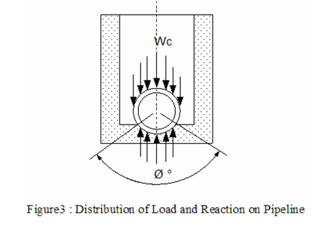
5. The Crossing Construction Type which is used to find the bedding constants for buried pipe (Kb & Kz), see Table V & Figure 3.
6. All the above information along with values for the following variables:
X – Longitudinal Distance over which Deflection Occurs (ft.)
Y – Vertical Deflection (in.)
Workflow
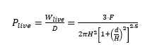
The pressure exerted on the pipe at pipeline depth due to a load at the surface can be calculated using Boussinesq’s equation:
(1)
where
![]() = pressure on the pipe due to the live load (psi)
= pressure on the pipe due to the live load (psi)
![]() = live load on the pipe (lb/in)
= live load on the pipe (lb/in)
![]() = diameter of the pipe (in)
= diameter of the pipe (in)
![]() = point load at the surface (lb)
= point load at the surface (lb)
![]() = depth of soil cover (in)
= depth of soil cover (in)
![]() = offset distance from the pipe to the line of application of the surface load (in)
= offset distance from the pipe to the line of application of the surface load (in)
Using this equation, a tire, track, or any other load with a known contact area can be represented by a series of point loads at the surface, and the total load on the pipe is calculated as the summation of the effect of the individual loads.
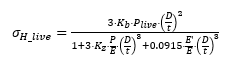
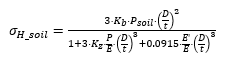
The CEPA equation combines the pressure stiffening and soil restraint terms into a single equation for determining circumferential (hoop) bending stresses due to live or soil loads:
 (2)
(2)
where
![]() = circumferential (hoop) bending stress due to the live load (psi)
= circumferential (hoop) bending stress due to the live load (psi)
![]() = soil parameter
= soil parameter
![]() = wall thickness (in)
= wall thickness (in)
![]() = soil parameter
= soil parameter
![]() = internal pressure (psig)
= internal pressure (psig)
![]() = Young’s modulus of elasticity for steel (30×106 psi)
= Young’s modulus of elasticity for steel (30×106 psi)
![]() = modulus of soil reaction (psi)
= modulus of soil reaction (psi)
and
 (3)
(3)
where
![]() = circumferential (hoop) bending stress due to the soil load (psi)
= circumferential (hoop) bending stress due to the soil load (psi)
The circumferential (hoop) stress due to internal pressure is given as:
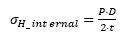 (4)
(4)
where
![]() = circumferential (hoop) stress due to internal pressure (psi)
= circumferential (hoop) stress due to internal pressure (psi)
The total circumferential stress, , is the sum of the stresses due to circumferential bending along with the hoop stress due to internal pressure. The total circumferential stress is compared to the allowable limit.
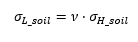
Internal pressure in pipelines restrained in soil causes a longitudinal stress equal to:
 (5)
(5)
where
![]() = longitudinal stress due to internal pressure (psi)
= longitudinal stress due to internal pressure (psi)
![]() = Poisson’s ratio for steel (0.3)
= Poisson’s ratio for steel (0.3)
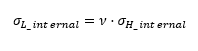
In a manner similar to the longitudinal stress from pressure, the soil load causes a longitudinal stress equal to:
 (6)
(6)
where
![]() = longitudinal stress due to soil load (psi)
= longitudinal stress due to soil load (psi)
The longitudinal stress due to the live load is determined as a combination of stress due to local bending and beam deflection. The calculation for the local longitudinal stress caused by the surface load is estimated using Bjilaard’s solutions for local loading on a pipe found in Roark’s Formulas for Stress and Strain .
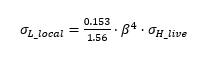 (7)
(7)
where
![]() = local bending stress (psi)
= local bending stress (psi)
and
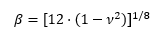 (8)
(8)
The vehicle load causes an axial pipeline deflection, which adds to the longitudinal stress due to internal pressure and temperature differential. If the pipeline is modeled as a beam on an elastic foundation, the maximum bending moment is given by Hetenyi1 as:
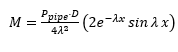 (9)
(9)
where
![]() = bending moment (in-lb)
= bending moment (in-lb)
![]() = Pressure on pipe from an equivalent point load (psi)
= Pressure on pipe from an equivalent point load (psi)
![]() = characteristic length (in-1)
= characteristic length (in-1)
![]() = distance along the pipeline (in)
= distance along the pipeline (in)
and
 (10)
(10)
where
![]() = bedding angle of pipe (degrees)
= bedding angle of pipe (degrees)
![]() = pipe moment of inertia (in4)
= pipe moment of inertia (in4)
is the uniformly distributed pressure on the pipe due to an equivalent point load at the surface that spreads at the soil distribution angle of 29.9 degrees from the surface point.
The longitudinal bending stress is given as:
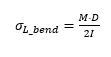 (11)
(11)
where
![]() = longitudinal bending stress (psi)
= longitudinal bending stress (psi)
The total longitudinal stress due to temperature differential is given as:
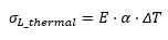 (12)
(12)
where
![]() = longitudinal thermal stress (psi)
= longitudinal thermal stress (psi)
![]() = coefficient of thermal expansion for steel (6.67×10⁻⁶ in/in deg F)
= coefficient of thermal expansion for steel (6.67×10⁻⁶ in/in deg F)
![]() = temperature differential (installation – operation)
= temperature differential (installation – operation)
The total longitudinal stress, , is the sum of the stresses from internal pressure, soil load, surface loads, axial deflection, and temperature differential. The total longitudinal stress is compared to the allowable limit.
The combined equivalent (Tresca – Equation 14; von Mises – Equation 15) stress is calculated as:
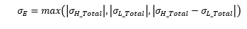 (13)
(13)
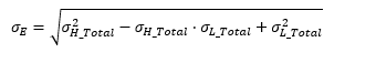 (14)
(14)
where
![]() = combined equivalent stress (psi)
= combined equivalent stress (psi)
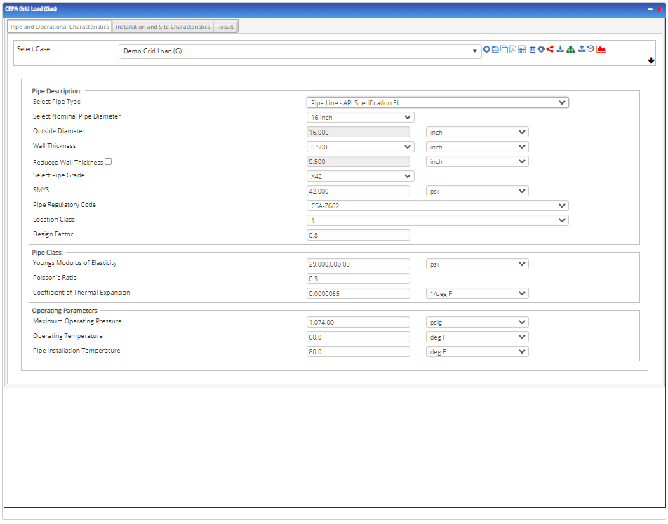
Input Parameters
- To create a new case, click the “Add Case” button
- Select the Track Load Analysis application from the Pipeline Crossing module.
- Enter Case Name, Location, Date and any necessary notes.
- Fill out all required fields.
- Make sure the values you are inputting are in the correct units.
- Click the CALCULATE button.
- Nominal Pipe Size(in):(1/8” – 48”)
- Pipe Outside Diameter(in):(0.625” – 48”)
- Pipe Wall Thickness(in):(0.068”- >2”)
- Pipe Grade
- SMYS
- Pipe Regularly Code
- Location Class
- Design Factor
- Youngs Modulus of Elasticity
- Poisson’s Ratio
- Coefficient of Thermal Expansion
- Maximum Operating Pressure
- Operating Temperature
- Pipe Installation Temperature
Installation and Site Characteristics:
- Soild Density
- Depth of Cover
- Bedding Angle
- Kb – Moment Parameter
- Kz – Deflection Parameter
- Soil Type
- Soil Compaction
- E Prime
- Vehicle Type
- Pavement Type
- Impact Factor
- Soil Load Equation
- Equivalent Stress Equation
- Pipe Regulatory Code
- Stress – Hoop
- Stress – Longitudinal
- Stress – Equivalent
- Vehicle Information
- Measurement Point X-Axis Coordinate
- Measurement Point Y-Axis Coordinate
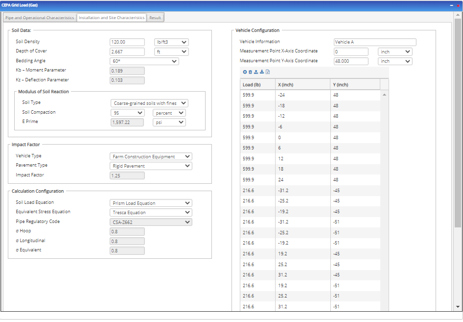
The CEPA Grid load calculation is intended for advanced users that wish to analyze a specific portion of a vehicle (e.g. a specific axle on a vehicle) or a custom vehicle type with a footprint (or ground contact area) which cannot be analyzed using one of the specific vehicle type tabs.
- Vehicle Information – Enter pertinent information about the vehicle (brand, model, year, etc.).
- Measurement Point X-coordinate – Enter the X-coordinate of the location where the program will calculate the pressure exerted on the surface of the pipe due to the vehicle load.
- Measurement Point Y-coordinate – Enter the Y-coordinate of the location where the program will calculate the pressure exerted on the surface of the pipe due to the vehicle load.
The “Grid INPUT” table was created to allow the user to define a grid of point loads matching the layout of their particular vehicle, instead of using one of the calculator’s default vehicle layouts. This tab enables the user to make a vehicle point load grid as simple or as complex as desired. This tab also allows the user to analyze a single axle on a particular vehicle or can be used for surcharge loads.
The three components of the grid input tab are the following:
- Load – Point Load (lb)
- X-coordinate (inch)
- Y-coordinate (inch)
Steps to enter the grid table entry
- Download the template for the grid table entry
- In the template START by creating a grid of point loads within each contact area of the vehicle wheels/tracks that represents the layout of the overall vehicle.
-
- NOTE: This could consist of a single point load located at the center of each wheel/track in the vehicle layout or it could be more complex and consist of many point loads distributed equally throughout the contact area of each wheel/track of the vehicle layout to mimic a surface pressure. See Figure 1 which shows the relation between Measurement Point “A” and the point loads at the center of each grid within the entire grid area.
- Each point load in a vehicle grid must be defined on the “Grid INPUT” tab by entering a value for “Load” (point load), “X” (which is the x-coordinate of the point load), and “Y” (which is the y-coordinate of the point load) in the respective input columns.
- NOTE: The reference origin, where (x, y) = (0, 0), is relative and its placement is user defined. It is essential that the reference origin remain the same for all coordinates utilized in the Grid INPUT tab analysis.
- NEXT the user must enter the coordinates for the Measurement Point (i.e. the location where the user wishes the program to calculate the pressure exerted on the surface of the pipe due to the vehicle load).
- THEN after the point load grid and the measurement point coordinates have been entered, save the file and upload the grid table to the program.
- NOTE: ALL columns, “Load”, “X”, and “Y” MUST contain a value for EACH point load, otherwise the program will return an error.

- View the results.
- If an input parameter needs to be edited be sure to hit the CALCULATE button after the change.
- To SAVE, fill out all required case details then click the SAVE button.
- To rename an existing file, click the SAVE As button. Provide all case info then click SAVE.
- To generate a REPORT, click the REPORT button.
- The user may export the Case/Report by clicking the Export to Excel/PowerPoint icon.
- To delete a case, click the DELETE icon near the top of the widget.
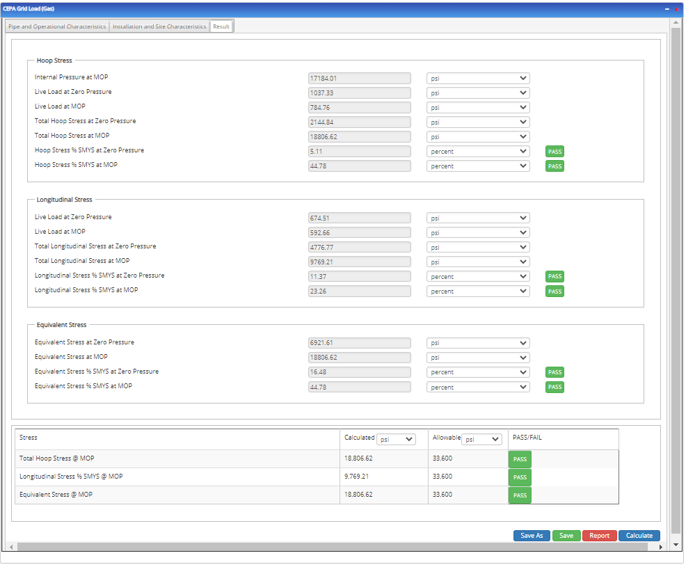
Hoop Stress:
- Internal Pressure at MOP
- Live Load at Zero Pressure
- Live Load at MOP
- Total Hoop Stress at Zero Pressure
- Total Hoop Stress at MOP
- Hoop Stress % SMYS at Zero Pressure
- Hoop Stress % SMYS at MOP
Longitudinal Stress:
- Live Load at Zero Pressure
- Live Load at MOP
- Total Longitudinal Stress at Zero Pressure
- Total Longitudinal at MOP
- Longitudinal Stress % SMYS at Zero Pressure
- Longitudinal Stress % at MOP
- Equivalent Stress at Zero Pressure
- Equivalent Stress at MOP
- Equivalent Stress % SMYS at Zero Pressure
- Equivalent Stress % SMYS at MOP
Results Table:
- Total Hoop Stress @ MOP
- Longitudinal Stress % SMYS @ MOP
- Equivalent Stress @ MOP