
Introduction
Darcy-Weisbach equations are valid for steady state flow. The friction factor – λ -depends on the flow, (laminar, transient, turbulent, Reynolds number) and the internal roughness of the pipe. The friction coefficient can be calculated by the Colebrook-White equation.
Limitations of this calculation depend on the flow regime for the right friction factor or coefficient.
Many factors affect the head loss in pipes, the viscosity of the fluid being handled, the size of the pipes, the roughness of the internal surface of the pipes, the changes in elevations within the system and the length of travel of the fluid.
H_L=f\bigg(\frac{L}{D}\bigg)\frac{v^2}{2g}
H_L=f\bigg(\frac{L}{D}\bigg)\frac{v^2}{2g}𝐻𝐿 − Head Loss [ft]
f – Friction Factor
𝐿 − Pipe Length [ft]
𝐷 − Internal Pipe Diameter [in]
𝑣 − Flowing Velocity [ft/sec]
𝑔 − Gravitational Constant [ft2/sec]
Friction factor is solved using Newton-Raphson method:
f=\frac{64}{Re};\,Laminar\,Flow: Re < 2000 \~\ \frac{1}{\sqrt{f}}=2\log_{10}(Re\sqrt{f})-0.8;\,Smooth\,Pipe:Re >4000\,and\,\frac{\varepsilon}{D}\rightarrow0\~\ \frac{1}{\sqrt{f}}=-2\log_{10}\biggr(\frac{\varepsilon}{3.7D}+\frac{2.51}{Re\sqrt{f}}\biggr);\,Transitional,\,Colebrook-White\,Eq,Re>4000\~\ \frac{1}{\sqrt{f}}=1.14-2\log_{10}\biggr(\frac{\varepsilon}{D}\biggr);\,Wholly \,Rough
f=\frac{64}{Re};\,Laminar\,Flow: Re < 2000 \\~\\ \frac{1}{\sqrt{f}}=2\log_{10}(Re\sqrt{f})-0.8;\,Smooth\,Pipe:Re >4000\,and\,\frac{\varepsilon}{D}\rightarrow0\\~\\ \frac{1}{\sqrt{f}}=-2\log_{10}\biggr(\frac{\varepsilon}{3.7D}+\frac{2.51}{Re\sqrt{f}}\biggr);\,Transitional,\,Colebrook-White\,Eq,Re>4000\\~\\ \frac{1}{\sqrt{f}}=1.14-2\log_{10}\biggr(\frac{\varepsilon}{D}\biggr);\,Wholly \,Rough𝑓 − Friction Factor
D – Inside Pipe Diameter[in]
𝜀 − Pipe Roughness[in]
Case Guide
Part 1: Create Case
- Select the Darcy – Weisbach application in the Hydraulics module.
- To create a new case, click the “Add Case” button.
- Enter Case Name, Location, Date and any necessary notes.
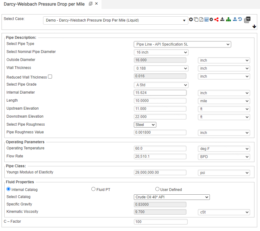
- Fill out all required parameters.
- Make sure the values you are inputting are in the correct units.
- Click the CALCULATE button to overview results
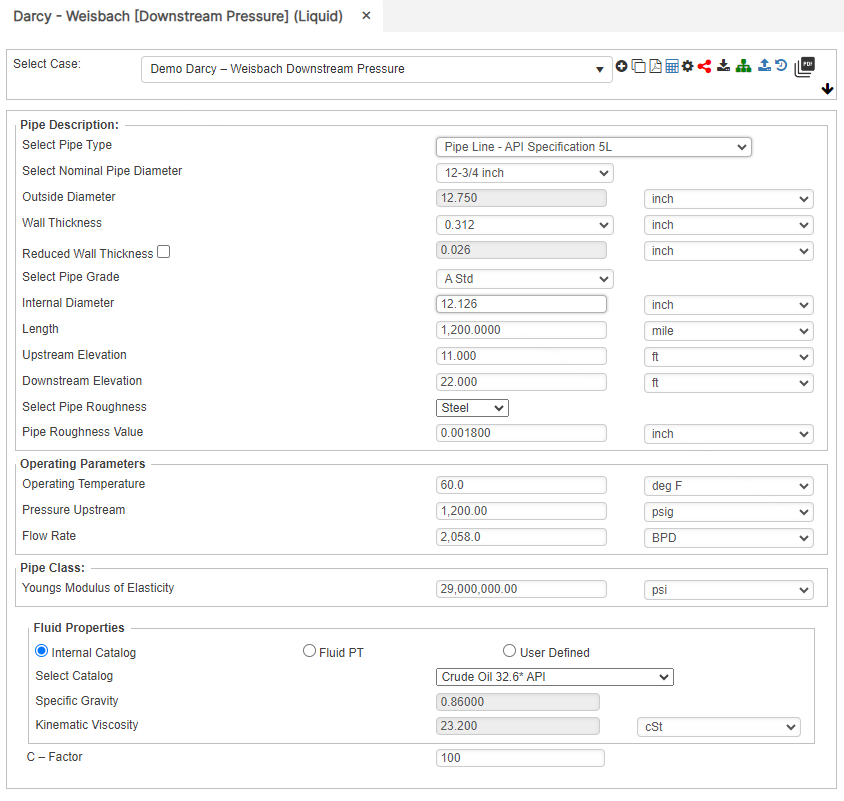
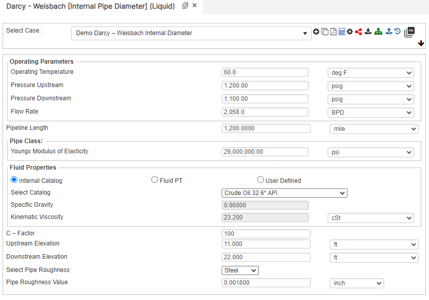
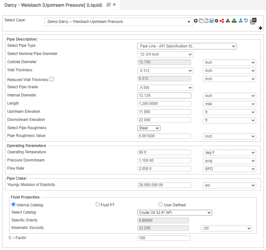
Input Parameters
- Temperature base(°F)
- Pressure base(psia)
- Gas Flowing Temperature(°F)
- Gas Specific Gravity
- Compressibility Factor
- Pipeline Efficiency Factor
- Upstream Pressure(psig)
- Downstream Pressure(psig)
- Flow Rate(Barrels per Day)
- Internal Pipe Diameter(in)
- Length of Pipeline(mi)
- Upstream Elevation(ft)
- Downstream Elevation(ft)
Downstream Pressure
Flow Rate
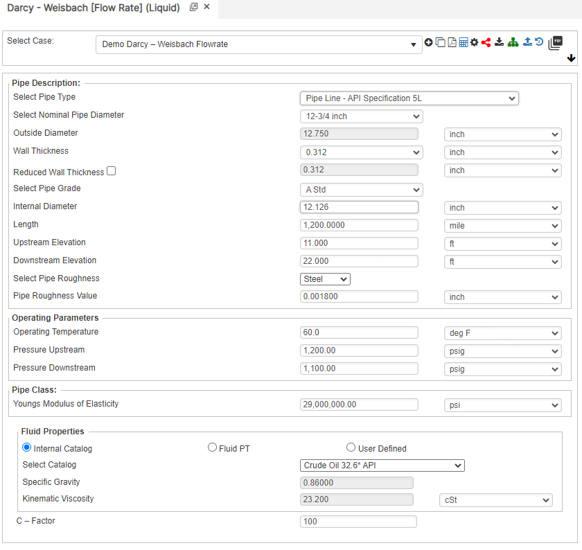
Internal Pipe Diameter
Upstream Pressure
Pressure Drop Per Mile
Part 2: Outputs/Reports
- If you need to modify an input parameter, click the CALCULATE button after the change.
- To SAVE, fill out all required case details then click the SAVE button.
- To rename an existing file, click the SAVE As button. Provide all case info then click SAVE.
- To generate a REPORT, click the REPORT button.
- The user may export the Case/Report by clicking the Export to Excel icon.
- To delete a case, click the DELETE icon near the top of the widget.
Results
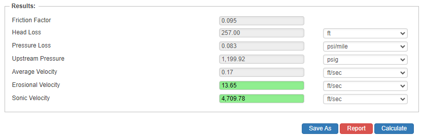
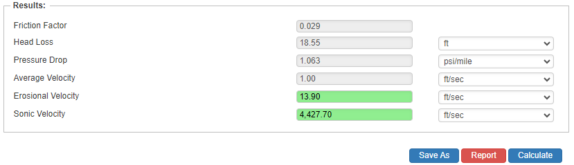
- Friction Factor
- Head Loss(ft)
- Pressure Loss(psi/mile)
- Flow Rate(Barrels per Day)
- Upstream Pressure(psig)
- Downstream Pressure(psig)
- Internal Pipe Diameter(in)
- Transmission Factor
- Velocity(ft/sec.)
- Erosional Velocity(ft/sec.)
- Sonic Velocity(ft/sec.)
Downstream Pressure

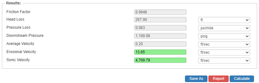
Flow Rate

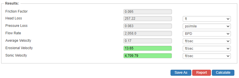
Internal Pipe Diameter

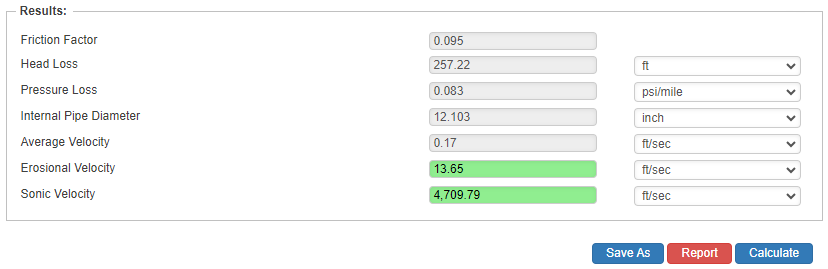
Upstream Pressure

Pressure Drop Per Mile

References
- “Pipeline Rules of Thumb” Gulf Professional Publishing, Seventh Edition, McAllister, E. W.
- “Gas Pipeline Hydraulics”, Systek Technologies, Inc., Menon, Shahi E.
- “Advanced Pipeline Design”, Carroll, Landon and Hudkins, Weston R.
- American Gas Association (AGA), “Reference: Eq-17-18, Section 17, GPSA”, Engineering Data Book, Eleventh Edition
- Hydraulic Transients, McGraw-Hill, New York., Streeter, V.L. and Wylie, E.B. (1967)
- Water Hammer Analysis. Jour. Hyd. Div., ASCE., Vol. 88, HY3, pp79-113 May, Streeter, V.L. (1969)
- Unsteady flow calculations by numerical methods’, Jour. Basic Eng., ASME., 94, pp457-466, June. Streeter, V.L. (1972),
- Hydraulic Pipelines, John Wiley & Sons, J. P Tullis (1989)
FAQ
-
What is Erosional Velocity?
Pipe erosion begins when velocity exceeds the value of C/SQRT(ρ) in ft/s, where ρ = gas density (in lb./ft3) and C = empirical constant (in lb./s/ft2) (starting erosional velocity). We used C=100 as API RP 14E (1984). However, this value can be changed based on the internal conditions of the pipeline. Check Out
-
What is Sonic Velocity?
The maximum possible velocity of a compressible fluid in a pipe is called sonic velocity. Oilfield liquids are semi-compressible, due to dissolved gases. Check Out