
Orifice Flow Equation
The accepted one-dimensional equation for mass flow through a concentric, square edged orifice meter is stated in the Equations below. The derivation is based on conservation of mass and energy, one-dimensional fluid dynamics, and empirical functions such as equations of state and thermodynamic process statements. Any derivation is accurate when all the assumptions used to develop it are valid.
As a result, an empirical orifice plate coefficient of discharge is applied to the theoretical equation to adjust for multidimensional viscous fluid dynamic effects. In addition, an empirical expansion factor is applied to the theoretical equation to adjust for the reduction in fluid density that a compressible fluid experiences when it passes through an orifice plate.
The fundamental orifice meter mass flow equation is as follows: q_m=C_dE_vY(\pi/4)d^2\sqrt{2g_c\rho_{t,p} \Delta P}
q_m=C_dE_vY(\pi/4)d^2\sqrt{2g_c\rho_{t,p} \Delta P}Where:
𝑞𝑚 − Mass Flow Rate
𝐶𝑑−Orifice Plate Coefficient of Discharge
𝑑 − Orifice Plate Bore Diameter (in)
𝐸𝑣 − Velocity Approach Factor
Δ𝑃 − Orifice Differential Pressure [in 𝐻20] at 60℉
𝜋 − Universal Constant = 3.14159
𝑌 − Expansion Factor
𝑔𝑐 − Dimensional Conversion Factor
𝜌𝑡,𝑝 − Density of the Fluid at Flowing Conditions (𝑃𝑓,𝑇𝑓)
The orifice meter is a mass meter from which a differential pressure signal is developed as a function of the velocity of the fluid as it passes through the orifice plate bore. Manipulation of the density variable in the equation permits calculation of flow rate in either mass or volume units. The volumetric flow rate at flowing (actual) conditions can be calculated using the following equation: q_v=q_m/\rho _{t,p}
q_v=q_m/\rho _{t,p}The volumetric flow rate at base (standard) conditions can be calculated using the following equation: Q_v=q_m/\rho _b
Q_v=q_m/\rho _b
The mass flow rate (𝑞𝑚) can be converted to a volumetric flow rate at base (standard) conditions (𝑄𝑣) if the fluid density at the base conditions (𝜌𝑏) can be determined or is specified.
Orifice Plate Bore diameter
The orifice plate bore diameter, d. is defined as the diameter at flowing conditions and can be calculated using the following equation: d = d_r \left(1 + \alpha_1(t_f – T_r)\right)
d = d_r \left(1 + \alpha_1(t_f - T_r)\right)
Where:
𝑑 − Orifice Plate Bore Diameter (in)
𝑑𝑟 − Mean Orifice Bore Diameter (in)
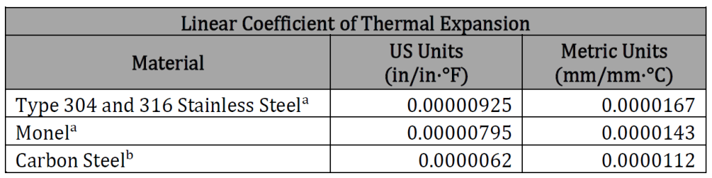
𝛼1 − Linear Coefficient of Thermal Expansion of Orifice Plate Material (in/in∙℉)
𝑡𝑓 − Flowing Gas Temperature (℉)
𝑇𝑟 − Reference Temperature Orifice Plates/Tubes (℉)
The meter tube internal diameter, D, is defined as the diameter at flowing conditions and can be calculated using the following equation: D = D_r \left(1 + \alpha_2(t_f – T_r)\right)
D = D_r \left(1 + \alpha_2(t_f - T_r)\right)
Where;
𝐷 − Meter Tube Internal Diameter (in)
𝐷𝑟 − Mean Meter Tube Diameter (in)
𝛼2 − Linear Coefficient of Thermal Expansion of Meter Tube (in/in∙℉)
𝑡𝑓 − Flowing Gas Temperature (℉)
𝑇𝑟 − Reference Temperature Orifice Plates/Tubes (℉)
Empirical Coefficient of Discharge Equation for Flange-Tapped Orifice Meters
The concentric, square-edged, flange-tapped orifice meter coefficient of discharge, 𝐶𝑑(FT), equation, developed by Reader-Harris/Gallagher (RG), is structured into distinct linkage terms and is considered to best represent the current regression data base. The equation is applicable to nominal pipe sizes of 2 inches (50 millimeters) and larger; diameter ratios (𝛽) of 0.1-0.75, provided the orifice plate bore diameter, d” is greater than 0045 inch (11.4 millimeters); and pipe Reynolds numbers (𝑅𝑒𝐷) greater than or equal to 4000.
C_d = C_i(FT) + 0.000511 \left( \frac{10^6\beta}{Re_D} \right)^{0.7} + (0.0210 + 0.0049A) \beta^4 C \~\
C_i(FT) = C_i(CT) + \text{Tap Term} \~\
C_i(CT) = 0.5961 + 0.2912 \beta^2 – 0.229 \beta^8 + 0.003(1 – \beta) M_1 \~\
\text{Tap Term} = \text{Upstream} + \text{Downstream} \~\
\text{Upstream} = [0.0433 + 0.0712e^{-6.01L_1} – 0.1145e^{-6.01L_1}](1 – 0.23A) B \~\
\text{Downstream} = -0.0116[M_1 – 0.52M_1^{1.3}] \beta^{1.1}(1 – 0.14A)
C_d = C_i(FT) + 0.000511 \left( \frac{10^6\beta}{Re_D} \right)^{0.7} + (0.0210 + 0.0049A) \beta^4 C \\~\\
C_i(FT) = C_i(CT) + \text{Tap Term} \\~\\
C_i(CT) = 0.5961 + 0.2912 \beta^2 - 0.229 \beta^8 + 0.003(1 - \beta) M_1 \\~\\
\text{Tap Term} = \text{Upstream} + \text{Downstream} \\~\\
\text{Upstream} = [0.0433 + 0.0712e^{-6.01L_1} - 0.1145e^{-6.01L_1}](1 - 0.23A) B \\~\\
\text{Downstream} = -0.0116[M_1 - 0.52M_1^{1.3}] \beta^{1.1}(1 - 0.14A)
Where:
𝛽 − Diameter Ratio = 𝑑/D
𝐶𝑑(𝐹𝑇) − Coefficient of Discharge at a Specific Reynolds number for Flange − Tapped Orifice Meter
𝐶𝑖(𝐹𝑇) − Coefficient of Discharge at infinite Reynolds number for Flange − Tapped Orifice Meter
𝐶𝑖(𝐶𝑇) − Coefficient of Discharge infinite Reynolds number for Corner − Tapped Orifice Meter
𝐿1 − dimensionless correction for the tap location
𝑒 − Napierian Constant = 2.71828
𝑁4 = 1.0 when D is in Inches = 25.4 when D is in millimeters
𝑅𝑒𝐷 − pipe Reynolds number
Reynold’s Number
The RG equation uses pipe Reynolds number as the correlating parameter to represent the change in the orifice plate coefficient of discharge, Cd, with reference to the fluid’s mass flow rate (its velocity through the orifice), the fluid density, and the fluid viscosity. The pipe Reynolds number can be calculated using the following equation: Re_D = 0.0114541 \frac{Q_b P_b G_r}{\mu D T_b Z_{bair}}
Re_D = 0.0114541 \frac{Q_b P_b G_r}{\mu D T_b Z_{bair}}
Where:
𝐷 − Meter Tube Internal Diameter (in)
𝑄𝑏 − Volume Flow Rate at Base Conditions (ft3/hr)
𝑃𝑏 − Base Pressure
𝑇𝑏 − Base Temperature (°R)
𝑍𝑏𝑎𝑖𝑟 − Compressibility of Air at 14.73 psia and 60℉
μ − Absolute Dynamic Viscosity (lbm/ft3)
𝐺𝑟 − Real Gas Relative Density
𝑅𝑒𝐷 − Pipe Reynolds number
Velocity of Approach Factor
The velocity of approach factor, 𝐸𝑣 , is calculated as follows:
\begin{align} E_v &= \frac{1}{\sqrt{1 – \beta^4}} \~\ \text{And, } \~\ \beta &= \frac{D}{ID} \end{align}
E_v = \frac{1}{\sqrt{1 – \beta^4}} \~\ \text{And,} \~\ \beta = \frac{D}{ID}
\begin{align*}
E_v &= \frac{1}{\sqrt{1 - \beta^4}} \\~\\
\text{And, } \\~\\
\beta &= \frac{D}{ID}
\end{align*}
Where:
𝛽 − Diameter Ratio
𝐸𝑣 − Velocity Approach Factor
𝑑 − Orifice Plate Bore Diameter (in)
𝐷 − Meter Tube Internal Diameter (in)
This assumption defines the expansion as reversible and adiabatic (no heat gain or loss). Within practical operating ranges of differential pressure, flowing pressure, and temperature, the expansion factor equation is insensitive to the value of the isentropic exponent. As a result, the assumption of a perfect or ideal isentropic exponent is reasonable for field applications.
The application of the expansion factor is valid if the following dimensionless pressure ratio criteria are followed:
\begin{align} 0&<\frac{\Delta P}{N_3P_{f1}}<0.2 \~\ \text{or, } \~\ 0.8&<\frac{P_{f2}}{P_{f1}}<1.0 \end{align}
\begin{align*}
0&<\frac{\Delta P}{N_3P_{f1}}<0.2 \\~\\
\text{or, } \\~\\
0.8&<\frac{P_{f2}}{P_{f1}}<1.0
\end{align*}
Where:
𝑁3 − Unit Conversion Factor
𝑃𝑓1 − Absolute Static Pressure at Upstream Tap (psi)
𝑃𝑓2 − Absolute Static Pressure at Downstream Tap (psi)
Δ𝑃 − Orifice Differential Pressure (in 𝐻20) at 60℉
Upstream/Downstream Expansion Factor
The upstream expansion factor requires determination of the upstream static pressure, the diameter ratio, and the isentropic exponent. If the absolute static pressure is taken at the upstream differential pressure tap, then the value of the expansion factor, 𝑌1 , shall be calculated as follows: Y_1 = 1 – \left(0.3625 + 0.1027 \beta^4 + 1.1328 \beta^8\right) \left[1 – \left(1 – x_1\right)^{\frac{1}{k}}\right]
Y_1 = 1 - \left(0.3625 + 0.1027 \beta^4 + 1.1328 \beta^8\right) \left[1 - \left(1 - x_1\right)^{\frac{1}{k}}\right]
When the upstream static pressure is measured, : x_1=\frac{\Delta P}{N_3P_{f1}}
x_1=\frac{\Delta P}{N_3P_{f1}}When the downstream static pressure is measured, : x_1=\frac{\Delta P}{N_3P_{f2}+\Delta P}
x_1=\frac{\Delta P}{N_3P_{f2}+\Delta P}Where:
𝑌1 − Upstream Expansion Factor
𝑁3 − Unit Conversion Factor
𝑥1 − Ratio of Differential Pressure to Absolute Static Pressure
𝑃𝑓1 − Absolute Static Pressure at Upstream Tap (psi)
𝑃𝑓2 − Absolute Static Pressure at Downstream Tap (psi)
Δ𝑃 − Orifice Differential Pressure [in 𝐻20]at 60℉
𝑘 − Isentropic Exponent
𝛽 − Diameter Ratio
The downstream expansion factor requires determination of the downstream static pressure, the upstream static pressure, the downstream compressibility factor, the upstream compressibility factor, the diameter ratio, and the isentropic exponent. The value of the downstream expansion factor, 𝑌2, shall be calculated using the following equation: Y_2 = \left[ 1 – \left(0.3625 + 0.1027\beta^4 + 1.1328\beta^8\right) \biggl{ 1 – \left(1 – x_1\right)^{\frac{1}{k}}\biggl} \right] \sqrt{\frac{P_{f1} Z_{f2}}{P_{f2} Z_{f1}}}
Y_2 = \left[ 1 - \left(0.3625 + 0.1027\beta^4 + 1.1328\beta^8\right) \biggl\{ 1 - \left(1 - x_1\right)^{\frac{1}{k}}\biggl\} \right] \sqrt{\frac{P_{f1} Z_{f2}}{P_{f2} Z_{f1}}}
When the upstream static pressure is measured, : x_1=\frac{\Delta P}{N_3P_{f1}}
x_1=\frac{\Delta P}{N_3P_{f1}}When the downstream static pressure is measured, : x_1=\frac{\Delta P}{N_3P_{f2}+\Delta P}
x_1=\frac{\Delta P}{N_3P_{f2}+\Delta P}Where:
𝑌1 − Upstream Expansion Factor
𝑌2 − Downstream Expansion Factor
𝑁3 − Unit Conversion Factor
𝑥1 − Ratio of Differential Pressure to Absolute Static Pressure
𝑥1/𝑘 − Upstream Acoustic Ratio
𝑃𝑓1 − Absolute Static Pressure at Upstream Tap (psi)
𝑃𝑓2 − Absolute Static Pressure at Downstream Tap (psi)
𝑍𝑓1 − Fluid Compressibility at Upstream Tap (psi)
𝑍𝑓2 − Fluid Compressibility at Downstream Tap (psi)
Δ𝑃 − Orifice Differential Pressure (in 𝐻20) at 60℉
𝑘 − Isentropic Exponent
𝛽−Diameter Ratio
Supercompressibility
In orifice measurement, 𝑍𝑏 and 𝑍𝑓1 appear as a ratio to the 0.5 power. This relationship is termed the supercompressibility factor and may be calculated from the following equation: F_{pv}=\sqrt{\frac{Z_b}{Z_{f1}}}
F_{pv}=\sqrt{\frac{Z_b}{Z_{f1}}}Base Pressure Factor
If contract base pressure differs from the reference base conditions (14.73 psia and 60℉), the initial calculated flow rate at reference base conditions will require conversion to the flow rate at the given base conditions. :F_{pb}=14.73psia /P_b
F_{pb}=14.73psia /P_bBase Temperature Factor
If contract base temperature differs from the reference base conditions (14.73 psia and 60℉), the initial calculated flow rate at reference base conditions will require conversion to the flow rate at the given base conditions. :F_{tb} = T_b/{519.67\,^{\circ}R}
F_{tb} = T_b/{519.67\,^{\circ}R}
Flowing Temperature Factor
F_{tf} = \sqrt{\frac{519.67\,^{\circ}R}{T_f}}
F_{tf} = \sqrt{\frac{519.67\,^{\circ}R}{T_f}}
Real Gas Relative Density Factor
F_{gr}=\sqrt{\frac{1}{G_r}}
F_{gr}=\sqrt{\frac{1}{G_r}}Numeric Conversion Factor
F_n=338.196E_v(D^2)(\beta^2)
F_n=338.196E_v(D^2)(\beta^2)
Flow Rate at Standard Conditions
Q_v = F_n \left(F_c + F_{st}\right) Y_1 F_{pb} F_{tb} F_{tf} F_{gr}F_{pv} F_{zb} \sqrt{{P_{f1} \Delta P}}
Q_v = F_n \left(F_c + F_{st}\right) Y_1 F_{pb} F_{tb} F_{tf} F_{gr}F_{pv} F_{zb} \sqrt{{P_{f1} \Delta P}}
Flow Rate at Base Conditions
Q_b = Q_v \left(\frac{P_s}{P_b}\right) \left(\frac{T_b}{T_s}\right) \left(\frac{Z_b}{Z_s}\right)
Q_b = Q_v \left(\frac{P_s}{P_b}\right) \left(\frac{T_b}{T_s}\right) \left(\frac{Z_b}{Z_s}\right)
Case Guide
Part 1: Create Case
- Select the AGA 3, Method II application from the Regulator & Meters Module
- To create a new case, click the “Add Case” button
- Enter Case Name, Location, Date and any necessary notes.
- Fill out all required Parameters.
- Make sure the values you are inputting are in the correct units.
- Click the CALCULATE button to overview results.
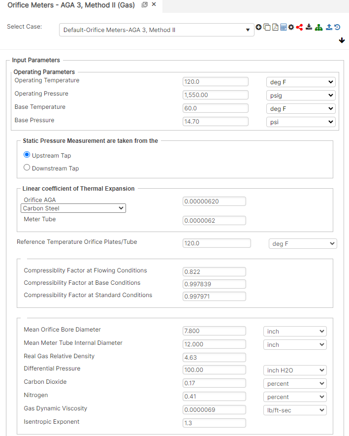
Input Parameters
- Operating Temperature (℉)
- Operating Pressure (psig)
- Base Temperature (℉)
- Base Pressure (psig)
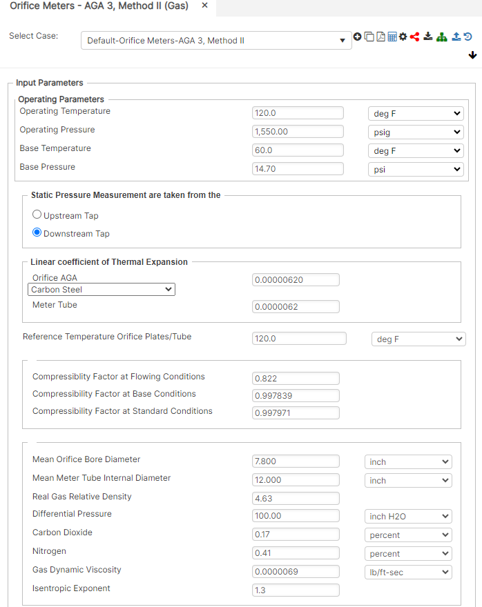
- Static Pressure Measurements (Upstream/Downstream)
- Linear Coefficient of Thermal Expansion
- Orifice AGA
- Meter Tube
- Reference Temperature Orifice Plates/Tube (℉)
- Compressibility Factor at Flowing Conditions
- Compressibility Factor at Base Conditions
- Compressibility Factor at Standard Conditions
- Mean Orifice Bore Diameter (in)
- Mean Meter Tube Internal Diameter (in)
- Real Gas Relative Density
- Differential Pressure [in H2O] at 60 deg F
- Carbon Dioxide (%)
- Nitrogen (%)
- Gas Dynamic Viscosity (lb/ft-sec)
- Isentropic Exponent
Upstream Tap
Downstream Tap
Part 2: Outputs/Reports
- If you need to modify an input parameter, click the CALCULATE button after the change.
- To SAVE, fill out all required case details then click the SAVE button.
- To rename an existing file, click the SAVE As button. Provide all case info then click SAVE.
- To generate a REPORT, click the REPORT button.
- The user may export the Case/Report by clicking the Export to Excel icon.
- To delete a case, click the DELETE icon near the top of the widget.
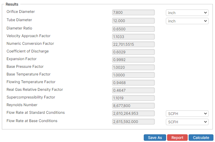
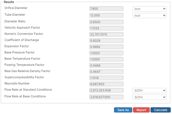
Results
- Orifice Diameter (in)
- Tube Diameter (in)
- Diameter Ratio
- Velocity Approach Factor
- Velocity Approach Factor
- Numeric Conversion Factor
- Coefficient of Discharge
- Expansion Factor
- Base Pressure Factor
- Base Temperature Factor
- Flowing Temperature Factor
- Real Gas Relative Density Factor
- Super compressibility Factor
- Reynolds Number
- Flow Rate at Standard Conditions (SCFH)
- Flow Rate at Base Conditions (SCFH)
Upstream Tap
Downstream Tap
References
- AGA Report No. 3 – Orifice Metering of Natural Gas and other Related Hydrocarbon Fluid – Parts 1-4