Flume Design – Rotational Method (Gas)

Estimating Roughness Coefficients

This section describes a method for estimating the roughness coefficient n for use in hydraulic computations associated with natural streams, floodways, and excavated channels. The procedures apply to the estimation of n in Manning’s formula. The coefficient of roughness n quantifies retardation of flow due to roughness of channel sides, bottom, and irregularities. Estimation of n requires the application subjective judgement to evaluate five primary factors:

• Irregularity of the surfaces of the channel sides and bottom
• Variations in the shape and size of the channel cross sections
• Obstructions in the channel
• Vegetation in the channel
• Meandering of the channel

Procedure for estimating n the procedure for estimating n involves selecting a basic value for a straight, uniform, smooth channel in the existing soil materials, then modifying that value with each of the five primary factors listed above. In selecting the modifying values, it is important that each factor be examined and considered independently.

Step 1. Selection of basic value of n. Select a basic n value for straight, uniform, smooth channel in the natural materials involved. The conditions of straight alignment, uniform cross section, and smooth side and bottom surfaces without vegetation should be kept in mind. Thus, basic n varies only with the material that forms the sides and bottom of the channel. Select the basic n for natural or excavated channels from Table 8.04a. If the bottom and sides of a channel consist of different materials, select an intermediate value. Table 8.04a. Basic Value of Roughness Coefficient for Channel Materials Soil Material Basic n.

• Channels in earth 0.02
• Channels in fine gravel 0.024
• Channels cut into rock 0.025
• Channels in coarse gravel 0.028

Step 2. Selection of modifying value for surface irregularity. This factor is based on the degree of roughness or irregularity of the surfaces of the channel sides and bottom. Consider the actual surface irregularity, first in relations to the degree of surface smoothness obtainable with the natural materials involved, and second in relation to the depth of flow expected. If the surface irregularity is comparable to the best surface possible for the channel materials, assign a modifying value zero. Irregularity induces turbulence that calls for increased modifying values. Table 8.04b may be used as a guide to selection of these modifying values. Table 8.04b. Modifying Value for Roughness Coefficient Due to Surface Irregularity of Channels Degree of Surface Comparable Modifying Irregularity Value.

• Smooth – The best obtainable for the material 0.000
• Minor Well-dredged channels – Slightly eroded or scoured side slope of canals or drainage channels 0.005
• Moderate Fair to poorly dredged channels – Moderately sloughed or eroded side slopes of canals or drainage channels 0.010
• Severe Badly sloughed banks of natural channels – Badly eroded or sloughed sides of canals or drainage channels; unshaped, jagged and irregular surfaces of channels excavated in rock 0.020

Source for Tables b-f: Estimating Hydraulic Roughness Coefficients

Step 3. Selection of modifying value for variations in the shape and size of cross sections. In considering this factor, judge the approximate magnitude of increase and decrease in successive cross sections as compared to the average. Gradual and uniform changes do not cause significant turbulence. Turbulence increases with the frequency and abruptness of alternation from large to small channel sections. Shape changes causing the greatest turbulence are those for which flow shifts from side to side in the channel. Select modifying values based on Table 8.04c. Table 8.04c. Modifying Value for Roughness Coefficient Due to Variations of Channel Cross Section.

• Character of Variation Modifying Value Changes in size or shape occurring gradually 0.000
• Large and small sections alternating occasionally, or shape changes causing occasional shift of main flow from side to side 0.005
• Large and small sections alternating frequently, or shape changes causing frequent shift of main flow from side to side 0.010-0.015

Step 4.

Selection of modifying value for obstructions. This factor is based on the presence and characteristics of obstructions such as debris deposits, stumps, exposed roots, boulders, and fallen and lodged logs. Take care that conditions considered in other steps not be double-counted in this step. In judging the relative effect of obstructions, consider the degree to which the obstructions reduce the average cross-sectional area at various depths and the characteristic of the obstructions. Shaped-edged or angular objects induce more turbulence than curved, smooth-surfaced objects. Also consider the transverse and longitudinal position and spacing of obstruction in the reach. Select modifying value based on Table 8.04d. Table 8.04d. Modifying Value for Roughness Coefficient Due to Obstruction in the Channel.

Relative Effect Modifying of Obstruction Value

• Negligible 0.000
• Minor 0.010 to 0.015
• Appreciable 0.020 to 0.030
• Severe 0.040 to 0.060

Step 5. Selection of modifying value for vegetation. The retarding effect of vegetation is due primarily to turbulence induced as the water flows around and between limbs, stems and foliage and secondarily to reduction in cross section. As depth and velocity increase, the force of flowing water tends to bend the vegetation. Therefore, the ability of vegetation to cause turbulence is related to its resistance to bending.

Note that the amount and characteristics of foliage vary seasonally. In judging the retarding effect of vegetation, consider the following: height of vegetation in relation to depth of flow, its resistance to bending, the degree to which the cross section is occupied or blocked, and the transverse and longitudinal distribution of densities and height of vegetation in the reach. Use Table 8.04e as a guide. Table 8.04e. Modifying Value for Roughness Coefficient Due to Vegetation in the Channel Vegetation and Flow Conditions Range in Modifying Value Comparable to:

• Low Effect 0.005 to 0.010 – Dense growths of flexible turf grass or weeds, such as Bermudagrass and Kentucky bluegrass. Average depth of flow 2 to 3 times the height of the vegetation.
• Medium Effect 0.010 to 0.025 – Turf grasses where the average depth of flow is 1 to 2 times the height of vegetation Stemmy grasses, weeds or tree seedlings with moderate cover where the average depth of flow is 2 to 3 times the height of vegetation Brushy growths, moderately dense, similar to willow 1 to 2 years old, dormant season, alongside slopes of channel with no significant vegetation along the channel bottom, where the hydraulic radius is greater than 2ft.
• High Effect 0.025 to 0.050 – Grasses where the average depth of flow is about equal to the height of vegetation Dormant seasons, willow or cottonwood tree 8-10-year-old, intergrown with some weed and brush; hydraulic radius 2 to 4 ft.
• Very High Effect 0.050 to 0.100 – Growing season, bushy willows about 1-yr old, intergrown with weeds in full foliage alongside slopes; dense grown of cattails or similar rooted vegetation along channel bottom; hydraulic radius greater than 4 ft Growing season, tree intergrown with weeds and brush, all in full foliage; hydraulic radius greater than 4ft.

Step 6. Computation of 𝑛^𝛿 for the reach. The first estimate of roughness for the reach 𝑛^𝛿, is obtained by neglecting meandering and adding the basic n value obtained in step 1 and modifying value from steps 2 through 5. : n_\delta=n+\sum\,modifying \,values

n_\delta=n+\sum\,modifying \,values

Step 7. Meander. The modifying value for meandering is not independent of the other modifying values. It is estimated from the 𝑛𝛿 obtained in step 6, and the ratio of the meandering length to the straight length. The modifying value for meandering may be selected from Table 8.04f. Table 8.04f. Modifying Value for Roughness Coefficient Due to Meander of the Channel Meander Ratio Degree of Modifying Meandering Value.

• 0.0 to 1.2 Minor 0.000 n
• 2.0 to 1.5 Appropriable 0.15 n
• 5.0 and greater Severe 0.30 n

Step 8. Computation of n for a channel reach with meandering. Add the modifying value obtained in step 7, to 𝑛^𝛿, obtained in step 6. The procedure for estimating roughness for an existing channel is illustrated in Sample Problem 8.04a. Sample Problem 8.04a. Estimation of roughness coefficient for an existing channel. Description of reach:

• Soil – Natural channel with lower part of banks and bottom yellowish gray clay, upper part light silty clay.
• Side slopes – Fairly regular; bottom uneven and irregular.
• Cross section – Very little variation in the shape; moderate, gradual variation in size. Average cross section approximately trapezoidal with side slopes about 1,5:1 and bottom width about 10 ft. At bank full stage, the average depth is about 8.5 ft and the avg. top width is about 35 ft.
• Vegetation – Side slopes covered with heavy growth of poplar tree, 2 to 3 inches in diameter, large willows, and climbing vines; thick, bottom growth of waterweed; summer condition with the vegetation in full foliage.
• Alignment – Significant meandering; total length of meandering channel, 1120 ft; straight line distance, 800 ft. Solution: Step Description Number n Value

Soil materials indicate minimum basic n 0.02
Modification for:

• Moderately irregular surface 0.01
• Change in size and shape judged insignificant 0.00
• No obstructions indicted 0.00
• Dense vegetation 0.08
• Straight channel subtotal, n = 0.11
• Meandering appreciable, meandering ratio: 1120/800 = 1.4 Select 0.15 from Table 8.04f
• Modified value = (0.15) (0.11) = 0.0165 or 0.02
• Total roughness coefficient n = 0.13

Out-of-Bank Condition Channel and Flood Plain Flow Work with natural floodways and streams often requires consideration of a wide range of discharges. At high stages, both channel and overbank or flood plain flow may occur. Usually, the retardance of the flood plain differs significantly from that of the channel, and the hydraulic computations can be improved by subdividing the cross selection and assigning different n values for flow in the channel and the flood plan. If conditions warrant, the flood plain may be subdivided further. Do not average channel n with flood plain n. The n value for in-bank flow in the channel may be averaged.

To compute a roughness coefficient for flood plain flow, consider all factors except meandering. Flood plain n values normally are greater than channel values, primarily due to shallower depths of flow. The two factors requiring most careful consideration in the flood plain are obstructions and vegetation. Many flood plains have dense networks of obstructions to be evaluated. Vegetation should be judged based on growing-season conditions.

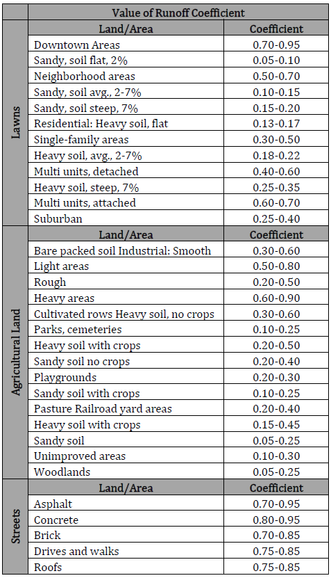
The overland flow can be estimated by calculating the average velocity in feet per minute and dividing the length (in feet) by the average velocity. Table 8.03a Value of Runoff Coefficient (C) for Rational Formula Land Use C Land Use C Business:

NOTE: The designer must use judgment to select the appropriate C value within the range for the appropriate land use. Generally, large areas with permeable soils, flat slopes, and dense vegetation should have lowest C values. Smaller areas with slowly permeable soils, steep slopes, and sparse vegetation should be assigned highest V value.

Calculations

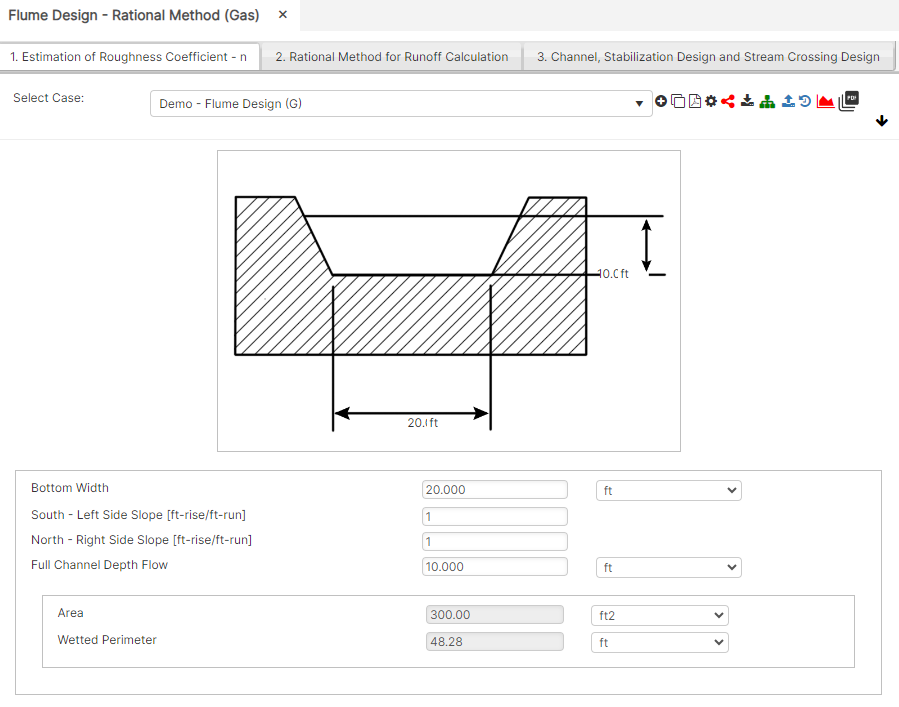
a=(\frac{H}{L_s})(\frac{H}{2})+(\frac{H}{R_s})(\frac{H}{2})+(Hb)

a=(\frac{H}{L_s})(\frac{H}{2})+(\frac{H}{R_s})(\frac{H}{2})+(Hb)

Where:
𝐿_𝑠 − South − Left side slope
𝑅_𝑠 − North − Right side slope
𝑏 − Bottom width (ft)
𝐻 − Full channel depth of flow (f𝑡)
𝑎 − Area of channel (ft²)

P_w=b+\sqrt{((\frac{H}{L_s})^2+H^2})+ \sqrt{((\frac{H}{R_s})^2+H^2)}

P_w=b+\sqrt{((\frac{H}{L_s})^2+H^2})+ \sqrt{((\frac{H}{R_s})^2+H^2)}

Where:
𝑃_𝑤 − Wetted Perimeter (ft)
𝑏 − Bottom width (ft)
𝐻 − Full channel depth of flow (𝑓𝑡)
𝐿_𝑠 − South − Left side slope
𝑅_𝑠 − North − Right side slope

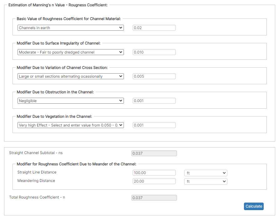
ns=n+F_{surface}+F_{size}+F_{obstruction}+F_{vegitation}

ns=n+F_{surface}+F_{size}+F_{obstruction}+F_{vegitation}

Where:
𝑛𝑠 − Straight channel subtotal
𝑛 − Basic Value for Roughness Coefficient for Channel Material
𝐹_{𝑠𝑢𝑟𝑓𝑎𝑐𝑒} = Modifier − Due to sand irregularity of Channel
𝐹_{𝑠𝑖𝑧𝑒} = Modifier − Due to variation of channel cross section
𝐹_{𝑜𝑏𝑠𝑡𝑟𝑢𝑐𝑡𝑖𝑜𝑛} = Modifier − Due to obstruction in the channel
𝐹_{𝑣𝑒𝑔𝑖𝑡𝑎𝑡𝑖𝑜𝑛} = Modifier − Due to vegetation in the channel

M_r=\frac{L_m}{L_s}

M_r=\frac{L_m}{L_s}

Where:
𝑀_𝑟 − Meandering Ratio
𝐿_𝑚 − Meandering distance
𝐿_𝑠 − Straight line distance

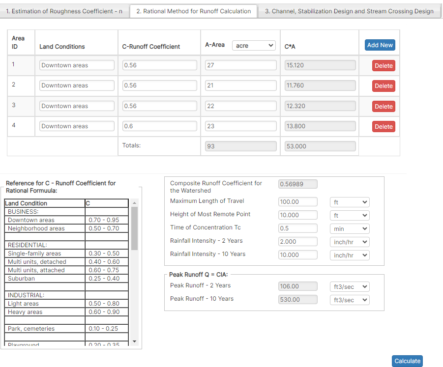
C_R=(CA){Total}/A{Total}

C_R=(CA)_{Total}/A_{Total}

Where:
𝐶_𝑅 − Composite Runoff Coefficient to the Watershed
𝐴_{𝑇𝑜𝑡𝑎𝑙} − Total Area (acres)
𝐶 − Runoff Coefficient
𝐴 − Area (acres)

Q_2=A_{Total}(I_2)(C_R) \~\ Q_10=A_{Total}(I_{10})(C_R)

Q_2=A_{Total}(I_2)(C_R) \\~\\ Q_10=A_{Total}(I_{10})(C_R)

Where:
𝐶_𝑅 − Composite Runoff Coefficient to the Watershed
𝐴_{𝑇𝑜𝑡𝑎𝑙} − Total Area (acres)
𝐼₂ − Rainfall Intensity − 2 Year (in/hr)
𝐼₁₀ − Rainfall Intensity − 10 Year (in/hr)
𝑄₂ − Peak Runoff − 2 Year (ft³/sec)
𝑄₁₀ − Peak Runoff − 10 Year (ft³/sec)

Q_{fb}=a(\frac{1.489}{n})((\frac{a}{P_w})^{0.667})(S^{0.5})

Q_{fb}=a(\frac{1.489}{n})((\frac{a}{P_w})^{0.667})(S^{0.5})

Where:
𝑎 − Area (ft²)
𝑛 − Basic Value for Roughness Coefficient for Channel Material
𝑃_𝑤 − Wetted Perimeter
𝑆 − Channel Slope
𝑄_{𝑑𝑒𝑠𝑖𝑔𝑛} = The Lesser of 𝑄₁₀ and 𝑄_𝑓𝑏

A_c=(\frac{H_f}{L_s})(\frac{H_f}{2})+(\frac{H_f}{R_s})(\frac{H_f}{2})+(H_fW_b)\~\ P_{wc}=W_b+\sqrt{((\frac{H_f}{L_s})^2+H_f^2})+ \sqrt{((\frac{H_f}{R_s})^2+H_f^2)}

A_c=(\frac{H_f}{L_s})(\frac{H_f}{2})+(\frac{H_f}{R_s})(\frac{H_f}{2})+(H_fW_b)\\~\\ P_{wc}=W_b+\sqrt{((\frac{H_f}{L_s})^2+H_f^2})+ \sqrt{((\frac{H_f}{R_s})^2+H_f^2)}

Where:
𝐴_𝑐 − Area of proposed channel (ft²)
𝑃_𝑤𝑐 − Wetted Perimeter of proposed channel (ft)
𝑁𝐿 − Select Manning Coefficient n for proposed lining
𝐻_𝑓 − Depth of flow (ft)
𝐿_𝑠 − South (Left) side − proposed
𝑅_𝑠 − North (Right) side − proposed
𝑊_𝑏 − Bottom width proposed (ft)
𝑆 − Channel Slope
𝑉_𝑑 − Design Velocity for Manning Equation
𝐴_𝑟 − Required area for Flume Pipe (ft²)

V_d=(\frac{1.489}{NL})((\frac{A_c}{P_{wc}})^{0.667})(S^{0.5})\~\A_r=Q_{design}/V_d

V_d=(\frac{1.489}{NL})((\frac{A_c}{P_{wc}})^{0.667})(S^{0.5})\\~\\A_r=Q_{design}/V_d

Case Guide

Part 1: Create Case

Input Parameters

• Channel Geometry Calculation
  • Width, Slope, Depth, Area
• Roughness Coefficient Calculation
  • Surface irregularity, variations, obstructions, vegetation, distance, and meandering
• Runoff Calculation
  • Runoff coefficient, height, time to concentration, rainfall intensity, and peak runoff
• Flow Conditions
  • Flow area, wetted perimeter, channel slope, Manning’s roughness coefficient, full bank

Part 2: Outputs/Reports

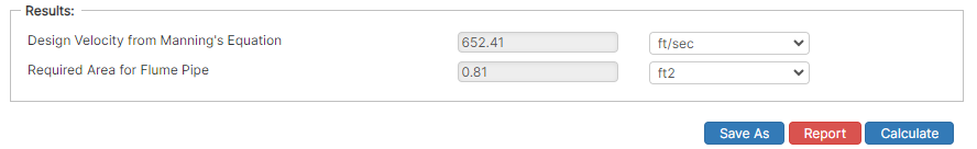
Results

• Design Velocity from Manning’s Equation (ft/sec)
• Required Area for Flume Pipe (ft²)

References

• ASME B31.8 – Gas Transmission and Distribution Piping Systems
• API 5L, API 5LS and API 5LX – Specification of Pipe Grade
• ASTM – Various – Weld Joint Factor
• CFR Code Part 192
• USDA-SCS Modified (Permissible Velocity of Water and Soil Erodibility)
• FHWA-HEC
• Pipeline Rules of Thumb Handbook
• Timoshenko, S – Theory of Elasticity Anchor Force

FAQ