
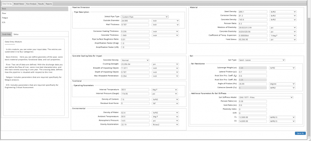
Basic Data
Basic Data view is shown in the figure below; the entry cells contain default values and units for each parameter.
Flowline Dimensions
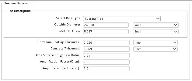
- Outer Diameter: The outside diameter of a steel pipe. The input value will be in the range of 75 mm to 1500 mm (3 in. to 60 in.)
- Wall Thickness: The wall thickness of the steel pipe. The input value should be smaller than 50 mm (2 in.)
- Corrosion Coating Thickness: The thickness of the corrosion coating around the steel pipe. Maximum allowable thickness is 200 mm (80 in.)
- Concrete Thickness: The thickness of the corrosion coating around the steel pipe. Maximum allowable value is 1250 mm (50 in.)
- Pipe Surface Roughness Ratio: External roughness ratio of the outermost surface of the pipe (k/D). Maximum allowable value is 0.1. Typical k/D values are:
- Concrete: Smooth Concrete Coating k/D = 10–³
- Roughened: Roughened Concrete Coating K/D = 10–²
- Very Rough: Further Roughened Pipe (typically resulting from soft bio-fouling) k/D = 5×10–²
- Drag and Lift Amplification Factors: The amplification factors on drag and lift coefficients are used when unusual pipe configuration or dimensions make the automatic selection of standard coefficients unreliable. This may be the case when bolt-on weights are used. The values of the standard coefficients are representative for a circular cylinder near a fixed boundary and are given in the Theory Manual. The default value is 1.0.
Material
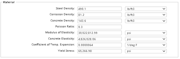
- Steel Density: The density of the pipe material (steel). The typical value is 7850 kg/m3 (490 pcf). The input value is limited to 15000 kg/m3 (1000 pcf).
- Corrosion Density: The density of the corrosion coating. The typical value is 1300 kg/m3 (81.2 pcf). The input value is limited to 8000 kg/m3 (500 pcf).
- Concrete Density: The density of the concrete (weight). The typical value is 2300 kg/m3 (143.6 pcf). The input value is limited to 8000 kg/m3 (500 pcf).
- Poisson Ratio: The density of the concrete (weight). The typical value is 2300 kg/m3 (143.6 pcf). The input value is limited to 8000 kg/m3 (500 pcf).
- Modulus of Elasticity: The modulus of elasticity of the steel pipe. The typical value is 200 GPa (29 Mpsi) in ambient temperature.
- Coefficient of Thermal Expansion: The thermal expansion coefficient of steel pipe. The input values should be in the range of 10-6 to 10-3 1/°C (5.6 × 10⁻⁷ to 5.5 × 10⁻⁴ 1/°F).
- Yield Stress: The yield stress of the steel pipe. The acceptable range for C-Mn steel grades 245 to 555 as per DNVGL-ST-F101 is 245 MPa to 675 MPa (35.5 to 97.9 ksi).
Functional
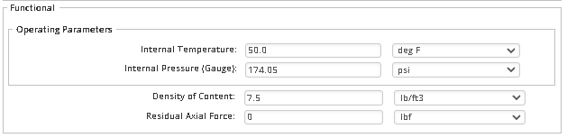
- Inner Temperature: The temperature of the pipe containment.
- Internal Pressure: Internal pressure of the pipeline.
- Density of the Content: Density of the pipeline containment. Maximum acceptable value is 3000 kg/m3 (187.3 pcf).
- Residual Axial Force: The residual axial force from installation.
Environmental
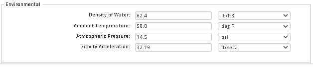
- Density of Water: The density of water. Typical value is 1000 kg/m3 (62.4 pcf) and the input is limited to maximum 1250 kg/m3 (78 pcf).
- Ambient Temperature: The temperature at the outer-side of the pipe.
- Atmospheric Pressure: This is a reference atmospheric, which is used to estimate the sandy soil-stiffness in the embankment.
- Gravity of Acceleration: Typical value is 9.81 m/s2 (32.2 ft/s2).
Soil
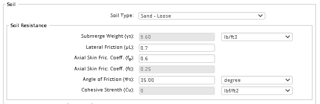
- Soil Type: Soil type determines the type of river-bed. A list of soil classes is available to select from. By selecting each soil class, the corresponding soil parameters are shown. Some of these parameters are pre-determined and read only (the colored ones). Also, some parameters are only available for sandy soils, while some are only available for clays. Note that all soil parameters would translate to static and dynamic soil stiffness, and soil resistance forces. The formulation used for sand and clay soils are different, hence the required parameters may vary. To define a fully-new soil with new parameters, select either ‘Sand-User Defined’ (which employs sand formulation) or ‘Clay-User Defined’ (to apply clay formulation).
- Submerged Weight (γs): Unit submerged weight of soil (value > 0). Unit submerged weight of soil is the ratio of the total weight of soil to the total volume of soil.
- Lateral Friction (μL): Lateral friction coefficient of soil (0< μL<1).
- Axial Skin Friction Coefficient (fϕ and fc): Skin friction factor of the soil/clay. This factor, together with friction angle, determines the axial friction coefficient of soil (greater than 0 and smaller than 1).
- Angle of Friction (φs): Friction angle of the soil/clay (between 0 and 90 degrees).
- Cohesive Strength (Cu): The undrained shear strength of soil (cohesive strength). Only applicable for clays (greater than 0).
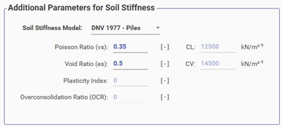
- Soil Stiffness Model: Two different soil model formulations are available to estimate static and dynamic soil stiffness:
- DNV 1997: This soil model is adopted from laterally loaded Piles. It considers the effect of cover height of soil above the pipe in the embankment of the soil stiffness.
- DNV-RP-F105: It adopts a simple estimation of soil stiffness. The value of the relevant parameters will be automatically applied based on the selected model but can be overridden if required. Irrelevant parameters become inactive upon selection of soil stiffness model.
-
- Poisson Ratio (νs): The Poisson ratio of soil (typical value 45).
- Void Ratio (es): The void ratio of soil (>0).
- Plasticity Index: The plasticity index of soil (only applicable to clays). It is used in the calculation of shear modulus of clays. The shear modulus determines the dynamic soil stiffness. Input value shall be between 0 and 100.
- Over-consolidation Ratio (OCR): The over-consolidation ratio (OCR) of soil (between 0 and 1).
- Lateral and Vertical Dynamic Soil Stiffness Coefficient (CL, Cv): A coefficient used to estimate the lateral/vertical dynamic soil stiffness. This coefficient is used when DNV-RP- F105 soil model is employed (<30,000 kN/m2.5 or 345,930 lbf/ft2.5).
Impact Data
For conditions where a concrete coating exists, an additional impact assessment is performed. The required information of this assessment is listed below. This data for concrete is only used for impact evaluation on concrete coating and it only comes into effect when the pipe is partially exposed (local impact). For details, please refer to the Theory Manual.
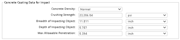
- Concrete Density: The density of the concrete; the available options are Normal and Light.
- Crushing Strength: The crushing strength of the concrete coating is from 3 to 5 times the cube strength for normal concrete density, and from 5 to 7 times the cube strength for lightweight concrete. The cube strength varies typically from 35 to 45 (5.1 to 6.5 ksi).
- Breadth and Depth of Impacting Object: Please refer to the Theory Manual for DNV-RP-F107
River Data
River discharge and river crossing data are shown in the figure below and described in this section. The integrity assessment of an exposed pipeline in a river channel requires the determination of:
- The river flow velocity at the location of the pipeline crossing.
- The forces on the pipeline induced by flow.
The local river flow velocity is normally related to the river discharge, which will display a large variation throughout the year. In many regions, there is a high spring flood when the snow melts. Autumn rains or other periods with concentrated rain may lead to another peak. Even over shorter periods of time, variations in discharge are considerable. Most rainy weather results in an increase in the flow unless the ground is very dry, or a number of upstream lakes or catchments may moderate the flow. By providing the number of events, and min/max values for river discharge, different conditions throughout a year can be assessed.
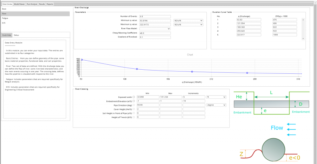
River Discharge
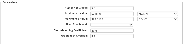
- Number of Events: Number of river events during a year (range: 0 – 12)
- Minimum Discharge (q) Value: The lowest discharge value during a year (range: 0 – 100 m3/s/m).
- Maximum Discharge (q) Value: The highest discharge value during a year (range: 0 – 100 m3/s/m).
- River Flow Model: River flow model relates the discharge value to the average velocity of river, depth of water in channel (river), slope of the channel, and riverbed roughness.
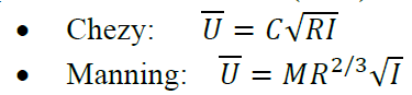
Where: 𝑈 is the average velocity of river, C and M are Chezy and Manning Coefficients, respectively, R is the depth of water, and I is the slope of the river.
- River Flow Model Coefficient: Depending on the selected flow model, the value represents Chezy or Manning Coefficient. The values of these coefficients depend on the river-bed roughness and the friction of the flow with the river-bed (value > 0)
- Gradient of Riverbed: Slope of the river (range: 0 – 1)
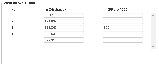
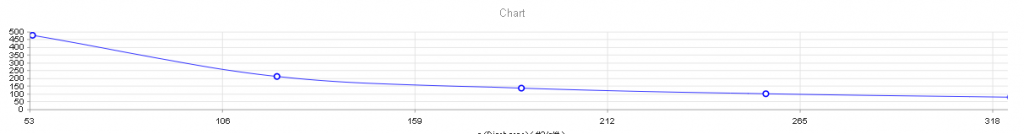
- Duration Curve Table: The table shows entrees for the river flow events. The discharge (q) is defined per unit width of the river, which is the specific discharge. Its unit is in m3/s/m (ft3/s/ft). The CPF(q)×1000 is the cumulative probability distribution of the discharge events assuming the total property be 1000. The probability density function PDF(q)×1000 is plotted against discharge rate.
River Crossing
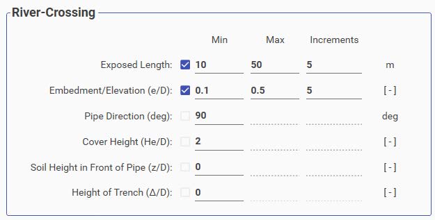
- Exposed Length: The length of the exposed section of pipeline. If assessments for multiple lengths within a range are required, the check box next to the field label should be ticked and minimum, maximum, and number of increments should be provided. Maximum allowable exposed length is 150 m (492 ft.). The number of increments should not exceed 10.
- Embedment/Elevation (e/D): Gap/embedment value; a positive value determines a gap between the pipe and river-bed, while a negative value determines how much of the pipe is buried. If assessments for multiple e/D values within a range are required, the check box next to the field label should bet icked and minimum, maximum, and number of increments should be provided. e/D should be in the range of 1 and -1. Maximum of 10 increments can be applied.
- Pipe Direction: The angle of a pipe with respect to river current (range: 0 – 90 degrees).
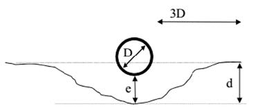
- Cover Height Ratio (He/D): Refer to the diagram below, this ratio determines the height of soil in the embankment that covers the pipe. The height is measured from top of the pipe (value > 0).
- Soil Height ratio in Front of Pipe (z/D): Refer to the diagram below. This ratio determines the height of soil in front of the pipe (range: 0 – 1).
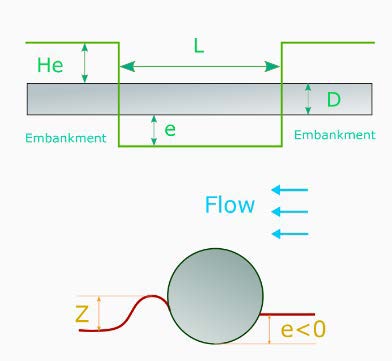
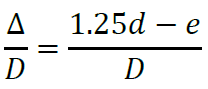
- Height of Trench ratio (Δ/D): Refer to the figure below. This ratio determines the depth of trench under the pipe (range: 0 – 1).
Fatigue Data
Fatigue Data module is shown in the figure below, followed by the details of the parameters.
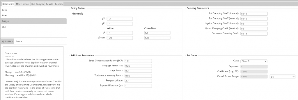
Safety Factors
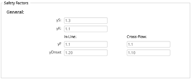
- γS : Safety factor on stress (value: 1.3).
- γK : Soil and structural damping safety factor; respectively 1.0, 1.15, 1.30 for low, medium and high safety classes, respectively.
- γF,IL : In-line natural frequency safety factor.
- γF,CF : Cross-flow natural frequency safety factor.
- γOn,IL : Onset of in-line VIV safety factor (value: 1.1).
- γOn,CF : Onset of cross-flow VIV safety factor (value: 1.2).
Damping
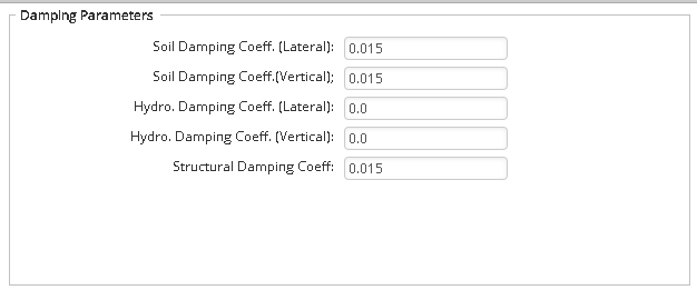
- Lateral Soil Modal Damping Ratio: Soil damping coefficient in lateral direction (range: 0 – 1). Typical value for screening purpose is 0.01.
- Vertical Soil Damping Ratio: Soil damping coefficient in vertical direction (range: 0 – 1). Typical value for screening purpose is 0.01.
- Lateral Hydrodynamic Damping Ratio: Hydro-dynamic damping coefficient in lateral direction (range: 0 – 1). Typical value for standard response is 0.0.
- Vertical Hydrodynamic Damping Ratio: Hydro-dynamic damping coefficient in vertical direction (range: 0 – 1). Typical value for standard response model is 0.0.
- Structural Damping Ratio: Structural damping coefficient. For pipelines with concrete coating, it is in the range of 0.01 – 0.02. If no information is available, 0.005 should be used.
Additional
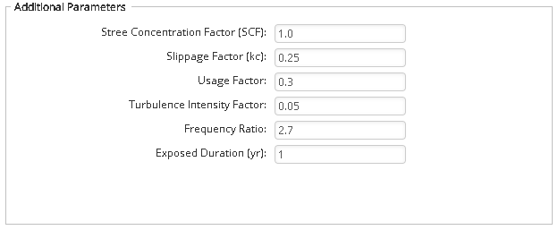
- Stress Concentration Factor (SCF): SCF due to potential geometrical imperfections in the welded area not implemented in the applied S-N curve. SCF should be calculated manually by the user and entered into the provided field. Minimum acceptable input is 1.0 (no concentration factor).
- Slippage Factor (kc): An empirical constant accounting for the deformation/slippage in the corrosion coating and the cracking of the concrete coating. The value of kc may be taken as 0.33 for asphalt and 0.25 for PP/PE coating.
- Usage Factor (η): A multiplier to the fatigue life to specify the allowable damage. For typical values, see the fatigue section in the Theory Manual. Range: (0-1).
- Turbulence Intensity Factor Over 30 Minutes: Turbulence intensity is the ratio between standard deviation of the velocity fluctuations and the steady current averaged over 10 min. or 30 min. This parameter is used to define a reduction factor applicable to the amplitude of VIV. If no specific information is available, a value of 5%. For further details, see DNVGL-RP-F105.
- Frequency Ratio: A frequency ratio of two consecutive vibrating modes. Please refer to DNVGL-RP-F105 and Theory Manual for typical values and range of applicability.
- Duration of Exposure: Total duration when the buried pipe was exposed in years.
S-N Curve
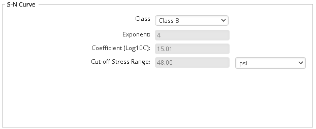
- S-N Curve: Available options include default S-N classes of B, C, D, E, F, F2, G, W, X, as we as the user defined. The S-N curve parameters will be updated based on the selected class. If user defined option is selected, the parameters should be entered manually. The S-N curves provided in the dropdown menu have been extracted from DNV 1977 (see Theory Manual). Should the user choose to use other data, the “user defined” option should be selected and the required parameters should be entered manually.
- Exponent: Fatigue exponent (the inverse slope of S-N curve) (Range: 1 – 5).
- Coefficient (Log10C): The coefficient in S-N curve (range: 1 – 30). C is characteristic fatigue strength constant defined as the mean-minus-two- standard-deviation curve.
- Cut-Off Stress Range: Threshold stress range where no significant fatigue damage occurs. Stress ranges smaller than the cut-off value may be ignored when calculating the accumulated fatigue damage.
ECA Data
The ECA Data module is shown in the figure below, followed by the details of each parameter.
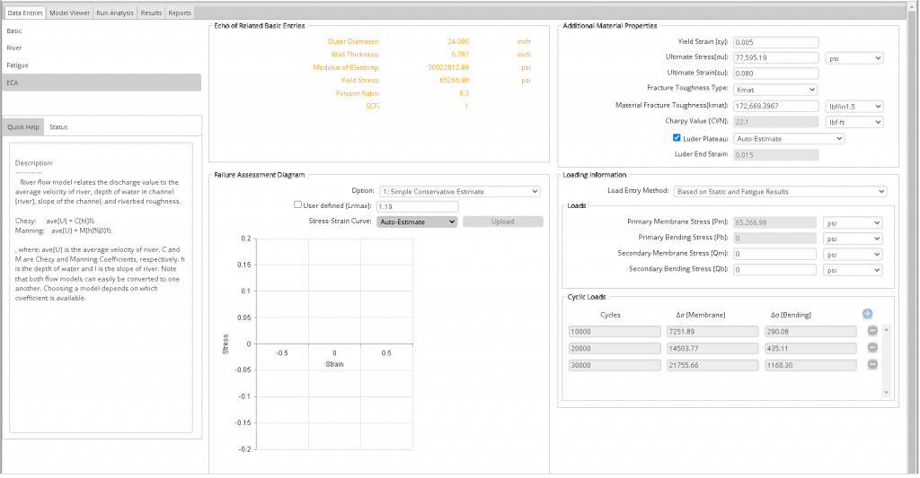
Material Properties
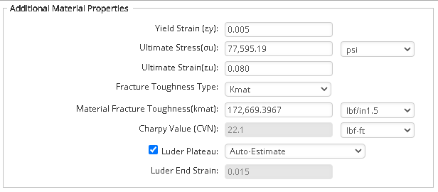
- εy: Strain at yield stress for pipeline steel. A value of 0.005 is usually used unless the exact value has been determined by tensile testing.
- σu: Ultimate tensile strength (UTS) of the pipe material. For DNV C-Mn steel grades 245 to 555 the acceptable values are 415 – 825 MPa (60.2 to 119.7 ksi).
- εu: Strain at tensile strength for pipeline steel. 0.08 is usually used in the absence of actual test data.
- Fracture Toughness: Type of material toughness parameter. Available options are Kmat and CVN.
- Kmat: Fracture toughness measured by stress intensity factor. The value depends on tensile proper-ties and CTOD. Typically equals to 6000 N/mm3/2 (172.67 kips/in5).
- CVN: Charpy V-Notch impact test absorbed energy (typical value: 30 J). Modern steels are usually above 100 J.
- Luder Plateau: To be ticked if the material stress-strain curve shows yield discontinuity. Available options are Auto and User Defined.
- Luder Strain Extent: The extent of the Luder plateau. Can be manually entered if User Defined Luder Plateau is selected (typically 0.02 to 0.03).
Failure Assessment Diagram (FAD)
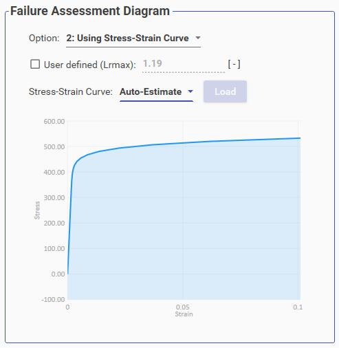
- Option: The assessment option according to BS7910. Available options are Option 1 and Option 2. For option 2, detailed stress-strain curve is required.
- User Defined Lr,max: The cut-off value for Lr in FAD (≥1.0). If check box is ticked, the user defined value is required, otherwise the cut-off will be calculated automatically.
- Stress-Strain Curve: The stress-strain curve of the pipe material. Available options are Auto and User Defined. If User Defined stress-strain curve is selected, the detailed curve data points shall be introduced using the “Load” button. The curve data shall be in .csv format with “Strain, Stress” heading with every data point in a separate line. The resultant stress-strain curve will be shown in the plot.
Echo of Related Basic Entries
The basic properties relevant to ECA (extracted from other sub=modules) are shown in this area.
Crack and Weld Geometry
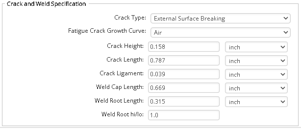
- Crack Type: The type and location of the crack in girth weld. Available options are:
- External surface breaking
- Internal surface breaking
- Embedded
- Fatigue Crack Growth Curve: Fatigue crack growth curve depends on the location of the flaw, coating, and environment. Available options are:
- In-air
- Marine
- Marine with -850mV cathodic protection (CP)
- Marine with -1100mV cathodic protection (CP)
- Crack Height: The height of flaw in girth weld. Maximum acceptable input value is approximately 85% of wall-thickness of the steel.
- Crack Length: The length of crack. Maximum acceptable input value is the circumference of the pipe.
- Crack Ligament: Remaining ligament for embedded flaws. Flaw recharacterization rule as per standard shall be considered.
- Weld Cap Length: The width of the weld cap which depends on joint preparation and whether it is mainline weld or repair weld.
- Weld Root Length: The width of the weld root which depends on joint preparation and whether it is mainline weld or repair weld.
- Weld Root hi/lo: The amount of displacement at the weld root which is specified in weld specification.
Loads
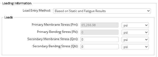
- Load Entry Method: Two types of load entry can be selected:
- Manual: The stresses are provided by the user.
- Auto: The stresses are taken from static and fatigue analysis. User should only input Qm and Qb values. ECA would be performed for all possible combinations of defined exposed lengths and gap-ratios.
- Primary Membrane Stress (Pm): Total membrane stress automatically calculated if Load Entry Method is Auto. For manual entry, primary membrane stress is assumed to be equal to nominal applied stress.
- Primary Bending Stress (Pb): Total bending stress automatically calculated if Load Entry Method is Auto. It is equal to nominal bending stress plus additional bending stress due to stress concentration factor. If manually entered, contribution of SCF shall be considered. If
 * SCF < Yield Stress then contribution of SCF equals to * (SCF-1); this value shall be added to the nominal bending stress (if present).
 - Secondary Membrane Stress (Qm): Total secondary membrane stress. Welding residual stress is usually treated as secondary membrane stress and conservatively assumed to be equal to yield stress.
- Secondary Bending Stress (Qb): Total secondary bending stress if known.
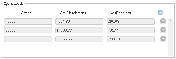
- Cyclic Loads: Fatigue loads automatically calculated if Load Entry Method is Auto. In manual entry mode, the values of each row (Cycles, Membrane, and Bending stress ranges) shall be provided by user. Rows can be added/removed using “+” and “-” buttons. Similar to static loads (see above), the contribution of SCF in bending stress ranges shall be considered.
Related Links
Table of Contents
Table of Pages
- Pipeline HUB User Resources
- AC Mitigation PowerTool
- API Inspector's Toolbox
- Crossings Workflow
- Horizontal Directional Drilling PowerTool
- Hydrotest PowerTool
- Pipeline Toolbox
- PRCI AC Mitigation Toolbox
- PRCI RSTRENG
- RSTRENG+
- Ad-hoc Analysis
- Database Import
- Data Availability Dashboard
- ESRI Map
- Report Builder
- Crossings Workflow
- Hydrotest PowerTool
- Investigative Dig PowerTool
- Hydraulics PowerTool
- External Corrosion Direct Assessment Procedure - RSTRENG
- Canvas
- Definitions