Static Results

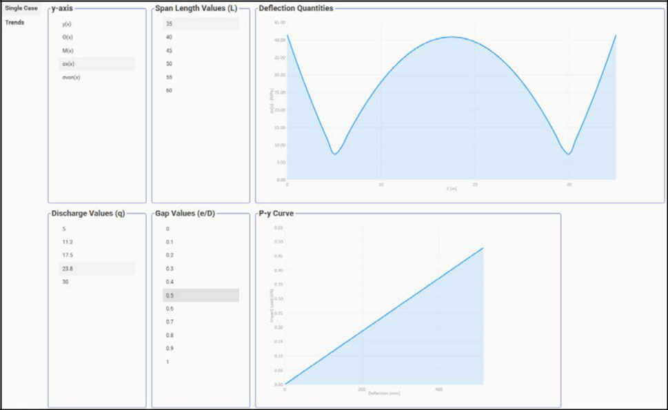
In this module, the results of static analysis are presented. An example of the static results is shown in the figure below.

Single Case Results

The results of the static analysis for different combinations of exposed length, discharge value, and gap size are shown in the Single Case tab.

The following functions are displayed in the top plot for the selected exposed length, discharge value, and gap size:

• y(x): displacement along the exposed length
• θ(x): slope deflection of the pipeline along the exposed length
• M(x): moment along the exposed length
• σx(x): stress in x direction along the exposed length
• σvon(x): von-mises stress along the exposed length 

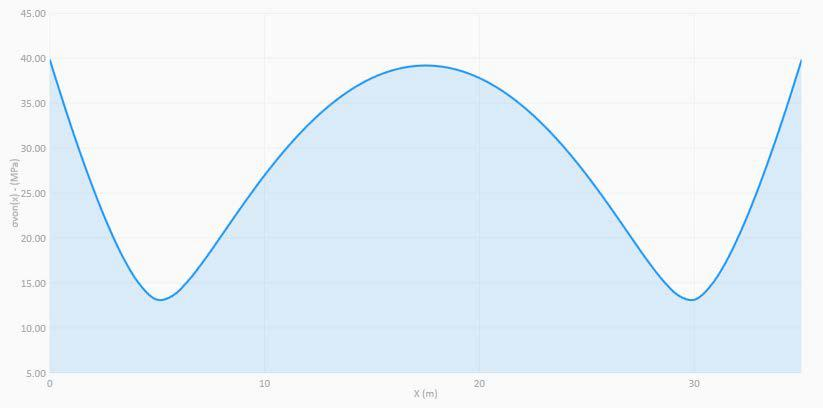
An example is shown in the figure below. The example shows von-mises stress along the exposed length (35 m) for discharge value of 30 and gap ratio of 0.5.

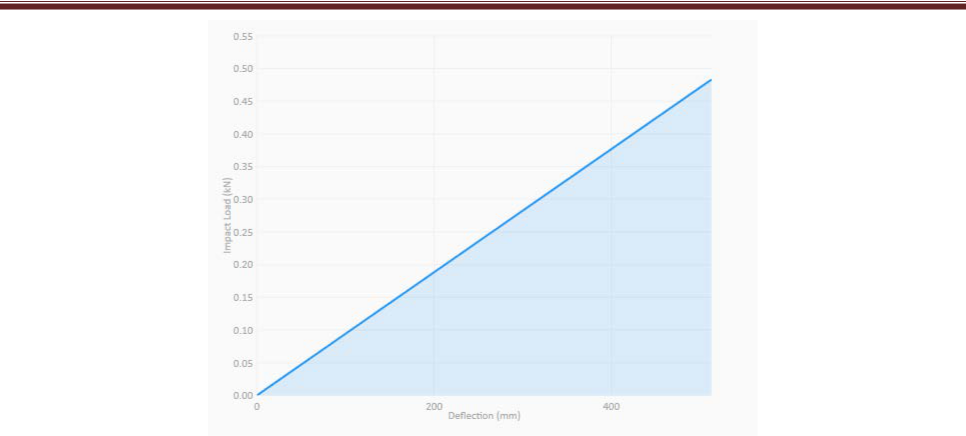
In the plot at the bottom of the single case static results, the results of the impact evaluation for the selected exposed length, discharge value, and gap sized is displayed (see figure below). The vertical axis of the plot is the impact load and the horizontal axis is the amount of deflection.

Trends

The trend plots are shown in the Trends tab, as shown in the Figure below.

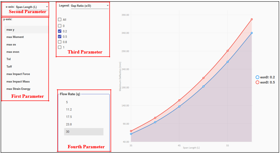
The following parameters can be selected as the vertical axis of the plots (first parameter).

• Maximum displacement
• Maximum moment
• Maximum longitudinal stress
• Maximum von-mises stress
• Non-linear axial tension
• Effective axial tension
• Maximum impact force
• Maximum impact mass
• Maximum strain energy

For the horizontal axis (second parameter), exposed length, flow rate, and gap ratio can be selected as the legend (third parameter).

For each value in the Fourth Parameter box (e.g. flow rate), multiple series can be displayed by ticking more items in the third Parameter box (see figure above).

Fatigue Results

Three tabs are available for fatigue analysis results: Response Model, Trend Plots, and Summary. Each tab is explained below.

Response Model

In-line and cross-flow response models for selected exposed length, gap size, and discharge values are displayed in the plots. The red data circles are representative of the selected parameters (see Figure below).

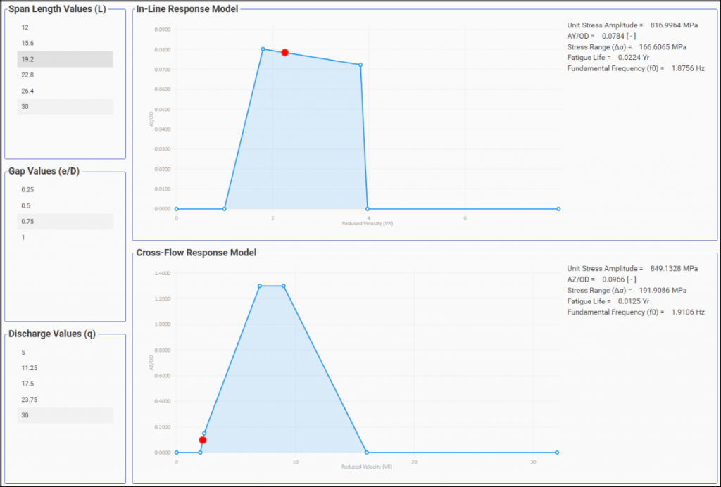
For each combination, additional results as listed below are also displayed at the left-hand side of the plots:

• Unit stress amplitude
• VIV amplitude (Ay and Az) to OD ratio
• Stress range
• Fatigue life
• Fundamental frequency

Trend Plots

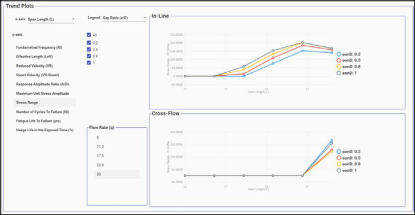
Similar to trend plots in static analysis results, fatigue trend plots display the trend of the following parameters as a function of exposed length, gap ratio, and flow rate.

• Fundamental frequency
• Effective length
• Reduced velocity
• Onset velocity
• Response amplitude ratio
• Maximum unit stress amplitude
• Stress range
• Number of cycles to failure
• Fatigue life
• Usage life in the exposed time

An example of trend plots is shown in the figure below.

Summary

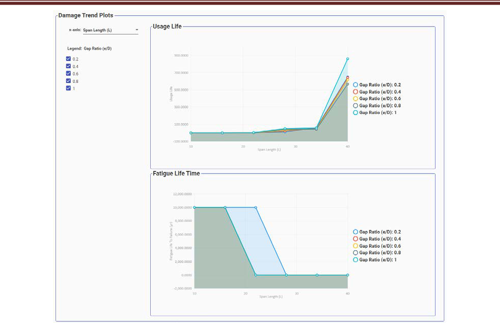
In the summary tab, usage life and fatigue life trend plots are displayed for selected exposed lengths and gap sizes as show in the Figure below.

ECA Results

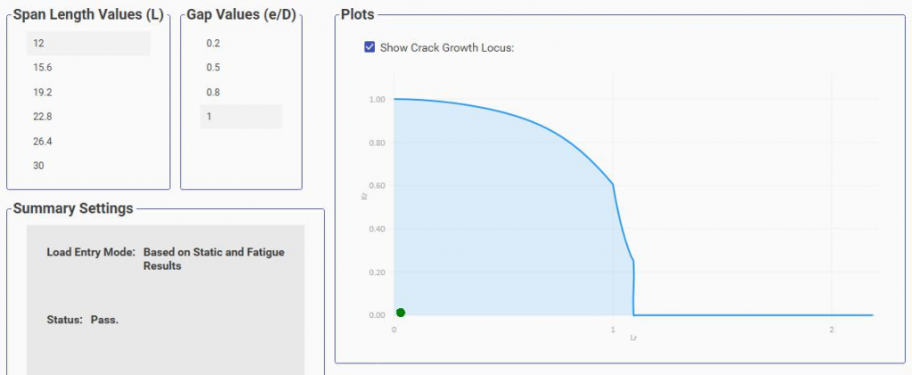
The ECA results are shown in the ECA Results Module. An example of the ECA results is shown in the Figure below. The assessment results for selected exposed length and gap value is displayed in the summary and plot sections.

Load entry mode and the final result of the assessment are shown in the summary section. Failure Assessment Diagram (FAD) along with the assessment points (green circles) are shown in the plots area.

Related Links