AC Mitigation PowerTool Theory Guide

Objective

Taking the same basic formula as the initial B31G criterion, but using the more accurate representation of Flow Stress, the modified Folias factor, and the effective area representation, a less conservative criterion was derived.

However, calculating failure stress using these factors is complex and cumbersome without a computer. It is for this reason the program RSTRENG was developed.

AC Inductive and Conductive Coupling

Electrical power lines carry an electrical current, leading to the production of a magnetic field from the conducting wire, inducing AC voltage on the buried pipe. This linking causes an alternating voltage and current to be induced onto a parallel collocated pipeline. When a pipeline is located near a power line, it is subject to several electrical effects depending on the operational status of the line. In addition, due to lightning strikes or other abnormal conditions, the power line can experience a short circuit condition known as a fault. To obtain data related to most major power lines in the United States, the Homeland Infrastructure Foundation-Level Data (HIFLD)website is available as is the AC Power Lines source here.

AC Pipeline Prediction Fundamentals

Understanding AC circuits and prediction fundamentals is critical to using the AC Mitigation PowerTool. The Technical Toolboxes website lists available training courses related to AC Interference and Mitigation. The AC Mitigation PowerTool focuses primarily on inductive and conductive (resistance) current and not on capacitive interference effects.

Electrostatic Interference:

• Capacitive when pipe is above ground
• Function of voltage not current
• Transfer of small amounts of power to pipeline
• Can result in high voltages on short sections
• Considered nuisance voltages

Electromagnetic Induced Voltages:

• Function of tower current, not voltage
• Power transfer is proportional
• Line current
• Longitudinal Electric Field (LEF)
• Length of parallelism
• Inverse to the separation distance
• Results in high voltages on long sections of pipeline

AC Faults – Inductive & Conductive

• Rare in the United States
• Short duration (micro to milliseconds)
• Weather conditions
  • High winds
  • Lightning
• Structural failure
  • Poor maintenance
  • Accidental damage
  • Vandalism/terrorism

AC Mitigation Understanding

AC mitigation is a way to reduce the effects of induced voltages from AC power line interference. Grounding calculations are derived from NACE CP Anode Types which can be found on the Pipeline Toolbox CP section.

Types of Mitigation or Grounding

• Discrete Anode (Single anode such as deep anode)
• Distributed Anode (Distributed Vertical and Horizontal Anode Strings)
• Linear wire or cable (Copper or Zinc)

AC Decoupling Devices

• Dairyland devices (See Appendix B)
• Copper cable for Parallel Grounding
• Distributed Anode Beds (Periodically Bonded to the Pipeline using Decouplers)
• Discrete Anode Beds

Mitigation to meet NACE Standards

• Less than 15VAC (Personnel Safety)
• Personnel Hazard
• IEEE-80

Gradient Control Mats (Personnel Safety)

• Appurtenances such as Test Stations & Valves
• Grid mats with Zn, Cu
• De-couplers

Practical Approach to Mitigating Corrosion

Induced AC Potentials

• Induced AC into a pipeline or to Earth is directly proportional to the strength of AC tower current load.
  • Inverse distance between parallel structures
  • Pipe diameter
  • Coating conductance/resistance
  • AC tower loads (Seasonal)
• Longitudinal electrical fields (LEF) are induced into the Earth.
• LEF can be field measured to estimate AC before a pipeline is constructed.

Discontinuities – Physical Pipeline

• Approaches or recedes from the power line R/W
• Changes distance from power line circuit
• Crosses under power line
• Contains an isolated device
• Transitions from below to above ground
• Significant coating resistance change

Discontinuities – Electrical Tower Line

• Power line transpositions
• Change in power line configuration
• Addition or removal of power line
• Changes in LEF (pipeline) at faulted tower

Tower Data

Additional data is required to determine the average tower ground resistance to remote earth and the average separation between the faulted transmission line towers (structures).

Cross sectional height and horizontal displacement of the shield (sky) wires from the tower center line are evident inputs. Program default accepts data for two wires with the assumption that the wires are periodically grounded to the tower grounds.

Physical placement of the wires, i.e. height and horizontal displacements from the tower center line, are evident when data is available. Default values for typical circuits as a function of circuit voltage levels are available from within the application database.

There are four (4) primary power transmission line types: (See Appendix C for Field Data Requirements)

• Single Horizontal
• Double Horizontal
• Single Vertical
• Double Vertical

The tower voltages run from 69 kV to 550 kV.  Example, if the tower voltages are lower than 69 kV, the 69 kV-100 can be used; however, the correct current load must be obtained from the power company or from the following as shown in the AC Inductive Theory Guide.

Power transmission operating data is not always available from power companies, or may be too expensive to obtain to fit the budget of the project. Although the application gives operating defaults, these values must be verified. especially in regards to day-to-day loads which directly impact the induced steady state voltages on the pipeline. Below is a table that shows the ranking of the current loads on a pipeline right of way.

Fault conditions from co-located power lines also present inductive/conductive conditions on the pipeline. Below, Table 2 provides typical tower voltages, currents and separation that are required for input into ACPT. This data should also be verified by the power company.

Bulk Soil Layering (Barnes Layer)

Barnes layer data is set up to represent the bulk soil multiple layers for the corrosive layer (pipe depth), apparent layer (steady state and inductive fault) and conductive layer (conductive fault). Other considerations include:

• Where soil resistivities are not deep and change, i.e. from deep tower footing grounds compared to the more shallow pipeline trench, faults may stress the coating.
• Where these conditions exist, multiple scenarios must be run at the fault tower(s) to assess for various depths.
• Using the Barnes Layer in areas where there are deep HDD crossings is recommended. Adjustment to spreadsheet calculations may be needed to accommodate these depths for more accurate assessments of these layers.
• In HDD crossings, it should be noted that drilling muds contain bentonite clays that have very low resistivities in the range of 100 ohm-cm. The soil resistivity meters may or may not detect this narrow layer of drilling muds around the pipe.
  • If the backfill is in typical soils, the drilling muds will migrate into the soil after several years.
  • If the backfill is in granite or similar rock, the muds may remain in place for many years.

Note: Barnes Layer – Below is a typical schematic of these three (3) major layers to consider bulk and specific layer resistivity. Any of these layers can be varied in depth depending on the geo layering and resistivity layers related to pipeline depth. There are soil resistivity inversion programs that calculate a two-layer method based on field measurements and depths. The ACPT allows the user to select the methods of measurement and calculation methods for data input.

The AC Mitigation PowerTool supports inputs from several methods of soil resistivity measurement.

• Apparent Resistivity (Deep) Layer should always be the deepest. The use of a minimum of a 100-foot depth or 30.5 meters is recommended to assess Inductive Faults and Steady State inductive voltages.
• Barnes Resistivity (Pipe) Layer should always be around the depth of the pipeline. Typical depths run from 3 to 6 feet or 1 to 2 meters except in the case of an HDD crossing. It is also used to calculate the current density of amps/m2.
• Conductive Resistivity Layer should always be the top surface player. Typical depths run from 3 to 10 feet or 1 to 3 meters. It is used to calculate conductive faults, step/touch potentials, and surface potentials or ground potential rise.

Example of Barnes Multi-layer Soil Resistivity Table

Note 1: Pin spacing can vary based on burial depth of pipe (feet or meters) and geotechnical information. Example: HDD Crossing 50′ depth for corrosive layer.

Note 2: If pin spacing is 5′, 10′, 15′, and 20′, use 5′ for corrosive layer and 10′ for conductive (surface layer).

Pipeline Data Required (Manual Entry)

• Pipe Diameter
• Coating resistance
• Depth of Cover per section
• Soil Resistivities
• Pipe Sections (Manual) = Use diagram below as reference
  • Angles should be like pipeline angles – i.e. section 1 (45 degrees ahead and to the left towards the power line). Section 3 (45 degrees ahead to the right).
  • Distances from pipe to tower should be based on which side of the pipe is relative to the power line. For example, section 1 is 50 feet from pipe to tower. Since there is a tower at section 2, it is the distance from pipe to tower (10 feet). Section 3 is -25 from pipe to the tower.
  • The same concept applies to the remaining line sections with section 4 being 45 degrees ahead to the left at -25 feet and section 5 being 45 degrees to the right at -75 feet.
  • Where long sections of pipe cross over from side of the power lines to the other, it may be necessary to change these to negative values as shown below.

Pipe Sections Creation

Four (4) ways to import Lat/Longs and GIS Data:

• Shape files (.shp)
• Map files (.kmz and .kml)
• Create from GIS
• Excel

Once a power transmission line and pipeline have been imported, users can create sections at nodes, towers, proposed mitigation sites, points of soil resistivity changes, transpositions, etc… See the User Guide for more detail on how to use the point and click feature to designate sections. Once this is completed, the user can calculate sections, distance, and angles. Once these angles have been calculated, the application will auto-populate the sections window.

The ACPT automatically calculates:

• Proximities to each structure
• Angles to each structure
• Section lengths based on engineering criteria
• Depth of cover (DOC) imported to each section as needed

Guideline for Determining Distance from Tower Leg to Pipeline

ACPT calculations are based on the centerline of the tower and pipeline (see example below).

• Conductive faults dissipate directly from tower grounds to earth onto the pipe (also called resistive faults and are of greater intensity).
• Inductive faults dissipate along the shield wires and grounds to earth. They are less intense than conductive faults.
• Pipeline distance for section fault 63.73 feet from center line of tower (calculated by ACPT)
• Arc distance calculated to 18.19 feet (calculated by ACPT) – must be calculated from the closest leg or legs of the tower.
  • Centerline distance of tower to closest leg to pipeline (measurement supplied by user) 25′.
• To determine if a fault condition is a threat using closest tower leg to the pipeline:
  • Calculate distance from centerline to pipeline (63.73′) minus user input closest leg (25′) = actual distance to pipeline (36.73′)
  • Calculate actual leg distance to pipeline (36.73′) minus arc distance (18.19′) = outside influence of arc distance (18.54′)

Guideline for Estimating Pipe Coating Resistance

The table below is used for estimating coating resistance quality. To perform an accurate assessment, the age, quality, and condition of FBE coating along with soil resistivity should be analyzed. How to assess quality:

• Excellent – Typically less than 2 years with no change in CP current demand
• Good – Typically 2 – 10 years and/or with small change in CP current demand
• Fair – Typically where the CP current demand has a moderate increase from original current requirement design
• Poor – Typically where the CP current demand has increased significantly with major coating deterioration and high CP demand

For more accurate coating assessments, it is recommended to run field tests for coating resistance or coating conductance. Also, see NAC Conductance test methods “Measurement of Protective Coating Electrical Conductance on Underground Pipelines.”

Note unit conversions in the table below.

• 1-ohm m = 100-ohm cm
• Coating resistance in Kohm-ft²

Not shown above: In low resistivity soil (2.5 ohm-m) with poor coating quality, to estimate coating resistance values use a multiplier of 0.1. Example: 2.5 ohm-m x 0.1 = .25 Kohm-ft². These are estimates and it is recommended to electrically test for actual coating resistance values.

Fault Puncture Resistance

To determine AC fault voltages that puncture underground pipe coatings, see table 5 below. These are estimates that are impacted by the condition of the coating.

AC Corrosion Rates

• Greatest at holidays having a surface area of 0.155 – 0.465 in² (1 – 3 cm²)
• High CP
• High Chloride and Alkaline environments
• DC current density rates greater than 1 am/m²

Note:  There are many factors that impact the AC corrosion rate from the size of the holiday, AC and DC current density, and the environment (resistivity and make up of soils).  Below is a NACE graph representing high and low likelihood of corrosion.

Mitigation

Most common mitigation approach is the grounding of the pipeline by means of buried horizontal wires, galvanic anodes, etc. This is for both Steady State and Faults. 

• Discrete (Ground Resistance at Node)
• Distributed (Single Anode Resistance) x (Spacing in Feet)
• Parallel (Linear Copper Cable(s) or Zinc with De-Couplers)
• Combinations of above (See Data Input Section 1 on Next Page for All 3 Types)
• Bonding (Pipe to Pipe in multiple pipe right-of-ways)

Discrete Grounds

Discrete grounding such as deep anodes can be used to mitigate widely spaced voltage peaks or nodes. Nodes start at the beginning of each section, typically where the pipe changes direction. If an isolating flange is located at the start/end of the line to a grounding station, or an isolated casing, a de-coupler can be used for a discrete ground to the station grounding across the isolating flange or casing to drain AC. A typical area of influence is approximately 500 ft. or 152.4 meters.

Note:  If Station Ground is used, Check Grounding for adequacy that does not to interfere with SCADA and or Operational Instrumentation.

Distributed Vertical or Horizontal Anode Strings

These anode strings are used at nodes or isolated voltage peaks.

Example: Assume a single vertical anode in a string that has a resistance to earth of 5 ohms for a 100-foot section length with a spacing of 250 feet between anodes. The input to program is 5 ohms x 250 feet spacing or 500 ohms-distance as a distributed ground. Decreasing the anode separation distance and increasing the anode length/size produces a more effective grounding system. This approach can be used when multiple closely spaced voltage peaks exist on the pipeline to isolate grounding form the CP system. Period grounding to the pipeline, i.e. 1500 feet or less, is recommended.

Linear (Parallel) Wire Long Line Copper Cable or Zinc Cable(s)

Linear parallel cables are typically used as a bonded horizontal cable, i.e. 1/0 or greater as the grounding element. This grounding system provides a very low impedance to ground which results in the lowest bound to achieve satisfactory steady state voltage levels. As an example, a 2000 foot section with a horizontal 2/0 copper cable is 0.22 ohms in a 5,000 ohm-cm soil using Sunde or Dwight’s calculations. The check box in the application defaults to zinc ribbon.

• Linear (parallel) copper grounding cables with or without backfill connected to Dairyland de-couplers have a history of good performance.
• Zinc ribbon grounding has been used in the past; however, limitations due to being part of the CP system have resulted in performance issues.

Combinations of Discrete, Distributed, and Parallel

All of these types of grounding can be used separately or in combination with each other. They are based on geometry of pipes and transmission lines and soil resistivity constraints.

See Appendix B Dwight’s Curve for grounding information for all types of the above mitigation. strategies.

Pipeline Bond Connections

Pipeline bond connections are used to develop pipeline grounding capabilities for both steady state and fault current mitigation. This approach is used when multiple closely spaced voltage peaks exist on the pipeline. However, voltage reduction is achieved with lowest mitigation resistance in grounding. Bonding is recommended at the start and end of each section or where pipelines are bonded together at valve stations, CP rectifiers, or other stations.

Example of Steady State/Current Density – Unmitigated

In the graph on the next page are the results for a 30-inch diameter line, FBE coated pipeline modeled with un-mitigated Steady State volts, amps, and current density. The calculated longitudinal electrical field (LEF) under the peak current conditions is 36.71 AC volts peak AC voltage in terms of the terminating current densities of 53.99 A/m². The field instantaneous measurement was 35 AC volts.  The modeled Steady State induced AC current in the pipeline ranged from 1.5 to 54 mA. The modeled AC values were based on an isolated pipeline system on each end.

The ACPT model produced the type of results that would be expected from this type of collocated pipeline and HVPL corridor. The length of the parallel configuration, the proximity between the pipeline and HVPL, the 2300 ohm-cm soil resistivity, and the new FBE pipeline coating are all significant contributors to the modeled AC voltage and current. Steady State condition calculated and modeled a maximum of 32 volts AC at the ends of the pipeline which exceeded the 15-volt safety limit. 

Where voltage safety is a concern for exposed or aboveground facilities, the use of grounding mats is recommended at test stations, above ground valve stems, risers, or other pipeline components. See Appendex A for more details. It should be noted that these types of facilities are to be considered separately from the ACPT program. These types of mitigation are for safety and are used to discharge fault type conditions during episodic events on the power lines. Secondary,  there may be some AC currents that are discharged that may help reduce Steady State Voltages.

Example of Steady State/Current Density – Unmitigated Graph

Example of Steady State/Current Density – Mitigated

The calculated longitudinal electrical field (LEF) under the peak current loading conditions 5.3 V AC for the entire pipe segment and the mitigated peak AC voltage in terms of the terminating impedances is 4 V AC. As would be expected, the ACPT model solution had the highest calculated AC voltages at either end of the pipeline. The modeled peak AC current in the pipeline ranged from 1 to 32 Amps.

The mitigated model using a discrete anode solution at each end and copper cable wire at peak voltages produced the type of results anticipated with the selected mitigation measures. It should be noted that steady state voltages and current densities are now within acceptable limits to stop corrosion.

Note: The calculated steady state modeled voltages at both ends of the pipeline are well within the desired 15-volt safety limit.

Example of Steady State/Current Density – Mitigated Graph

Fault Voltage and Current – Unmitigated

Fault condition analysis was performed at several tower locations to determine the most severe condition. This severe fault condition was modeled at the end of the line where it crosses the tower lines. A maximum threshold AC voltage across the coating was modeled at 2,700 AC volts. It would require more than 14,000 volts for a 14-mil thick coating for the risk of coating damage. Based on the fault condition model results as shown below, it did require additional AC mitigation measures (discrete anode) to reduce the fault condition AC voltages for safety.

In addition, the arc radius and surface, step and touch potentials were calculated.

The results of the peak fault voltages and currents that were modeled are displayed below. Note the difference from a maximum fault on the tower to the pipeline. The graph represents the middle of the line as being the highest risk.

Fault condition analysis was performed at several tower locations to determine the most severe condition. This severe fault condition was modeled at the end of the line where it crosses the tower lines. A maximum threshold AC voltage across the coating was modeled at 2,700 AC volts. It would require more than 14,000 volts for a 14-mil thick coating for the risk of coating damage. Based on the fault condition model results as shown on the next page, it did require additional AC mitigation measures (discrete anode) to reduce the fault condition AC voltages.

Note the difference from a maximum fault on the tower to the pipeline. The graph represents the middle of the line as being the highest risk.

In addition, the arc distance, surface, step, and touch potentials were calculated for above ground appetences.

Note:  When touch, step, and surface potentials do not meet electrical codes for safety, they are primarily mitigated using off line calculations for above ground appetences such as risers, valves, spans, test stations etc. to protect personnel working  on or around these facilities.  Whereas fault voltages and currents are mitigated for the underground pipeline and coating using the ACPT program.

Example of Fault Voltage and Current with Mitigation

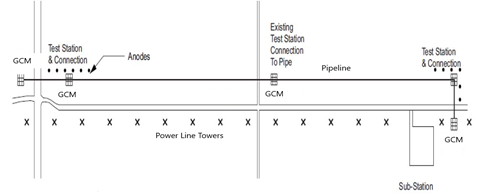
This project required a distributed anode bed on each end of the pipeline system to reduce the effects of faults where the pipeline crossed AC tower line (See pictorial below). For personnel safety, it is recommended to use gradient control mats (GRMs) at all above ground appurtenances such as test stations and values (See Appendex A for details). In addition, solid state de-couplers were recommended at each of these gradient control mat sites to isolate the CP system from the grounding. The number of anodes were determined by NACE ground bed calculations for a single anode to earth and the appropriate distributed spacing. 

In addition, Technical Toolboxes has a module and application in the Pipeline Toolbox HUB, Corrosion Control and Cathodic Protection with several applications for calculating vertical and horizontal anode(s) to earth. This module also has an application for single (copper wire or zinc) linear/parallel anodes or grounds to earth.

On the next page is linear copper grounding system (Dashed Blue Lines) with decoupler located at a fault area (Orange Dot). Using the ArcGIS map in conjunction with planning the type of mitigation that can be installed allows the designer to make faster engineering assessments to mitigate the effects of the AC fault voltage peaks and high AC current.

AC Mitigation Design Using a Parallel Anode/Grounding System

Below are the mitigation results for fault voltage and current. The calculated fault voltage 1,150 VAC on the coating surface that is below the effects for damage to occur based on a 5,000 VAC criterion. However, it should be noted that the surface, touch, and step potentials can present a safety risk to personnel, should a fault occur at that milli-second in time during episodic conditions. Therefore, it is always recommended to use gradient control mats for any above ground appurtenances even with mitigation for personnel safety. Good safety practices should be implemented whenever electrical storms are in the vicinity of these facilities.

Graph of Fault Voltage and Current – Mitigated

Disclaimer: Conductive Mitigated Voltage is Calculated using a PRCI Approach.

AC Corrosion Calculations

Current Density

• High AC current density has resulted in AC corrosion.
• AC modeling and mitigation is used to estimate AC voltage and AC current densities.
• AC current density can be calculated using a known area on a coupon (See Appendix D).
• Where:
  • i_AC = AC Current Density (A/m²)
  • V_AC = pipe AC voltage to remote earth (volt)
  • ρ = soil resistivity (ohm-m)
  • d = diameter of a circular holiday
• AC voltages as low as 1 VAC can produce high current densities at 1 sq. cm. (.01128″) holiday in lower resistivity areas.
• AC voltage required for a current density of 100 A/m2 is 100 ohm-cm soil at a 1 sq. cm. (0.01128″) holiday is:

Note: This calculated AC voltage is extremely low. The reason that this extreme case was shown is because it happened in a brackish water crossing where a product leak occurred on a pipeline. The brackish water resistivity averaged 30-ohm cm. This case shows the importance of understanding the risk factors and environmental conditions around the pipe.

Below is an AC chart representing these types of calculations.

Risk of AC Corrosion Voltage Versus Resistivity

Where AC current density is above 100 A/m2, the likelihood of AC corrosion can occur. It can also occur at lower values based on DC current density and other factors. Most engineers agree that at less than 30 A/m2 it does not occur. Below is a graph showing another version of the above graph with multiple ranges. 

In addition, the 15 VAC Shock Hazard Limit is shown.

Note: See NACE documents SP0177 Latest Edition Safety Considerations and NACE 35110 State of the Art on AC Considerations for more information.

Summary

The format developed for this AC Mitigation program makes most of the computational functions and much of the data input very easy for the designer, thus making these results understandable way for unlimited pipelines and transmission towers.  This is the first in this area of complex mathematical modeling.  For example, data input for only one computer screen is required to exercise the program to assess the following including reporting.

• Steady state voltage and current induction predictions
  • Current density predictions
• Fault voltage and current induction predictions
• Step, Touch and Surface Potentials (Personnel Safety)
• Mitigation
  • Discrete
  • Distributed
  • Parallel
• Barnes Layer (Bulk Soil Resistivity Layers)
  • Surface
  • Barnes
  • Apparent
• Depth of Cover (DOC)
• Report Generation
  • PDF
  • Spreadsheets

The AC Power Tool is an easy-to-use interface that makes the use of a HUB based program as viable tool for several potential users in your company. All pipeline functions are connected using Technical Toolboxes ArcGIS or your company’s ArcGIS.

References

1. PR-200-9414 AC Predictive and Mitigation Techniques – Final Report
2. NACE SP0177 Latest Edition Safety Considerations
3. NACE 35110 State of the Art on AC Considerations
4. NACE Technical Committee Report, “Mitigation of Alternating Current and Lightning Effects on Metallic Structures and Corrosion Control Systems”

Appendices

• Appendix A – AC Mitigation System Checklist by Dairyland
• Appendix B – Dwight’s Grounding Chart
• Appendix C – Field Data Requirements
• Appendix D – Underground AC/DC Coupons for Monitoring

Appendix A

– Dairyland AC Mitigation System Checklist

Inductive voltage mitigation equipment:

• De-coupler
• Grounding material (bare copper, zinc, etc…)
• Isolated conductors connecting de-coupler and grounding material
• Conductor attachment method: thermite welding, pin brazing, plus coating/sealing system
• Enclosure or pedestal for de-coupler
• Disconnection means for de-coupler testing or close internal surveys (isolations witch). Select switch with AC steady state and AC fault ratings equal to the de-coupler ratings.

Measurement equipment:

• Test station
• Coupon for AC current density measurement (or multiple function coupon)

Step and touch voltage near above-grade structures and connections:

• Gradient control mats
• Thermite welding molds/charges
• Anode for mat protection
• De-coupler for zinc grounding mat isolation from pipeline
• Isolated conductor

Isolating joint protection – subject to AC induction:

• De-coupler
• De-coupler mounting brackets appropriate for insolated join type

Application Notes for AC Mitigation

• Select AC fault current rating that exceeds modeled or calculated values expected on pipeline.
• Select standard AC steady state current rating unless modeled or measured conditions require the higher 80A PCR rating.
• Most AC mitigation sites are classified as Div. 2/Zone 2 or are “ordinary” locations. Div. 2/Zone 2 products will cover either. If Div. 1/Zone 1 ratings are needed, use model PCRH.
• Apply product environmental ratings suitable for site location. Most are typically above grade and not subject to flooding. IF below grade, select IP68 or NEMA 6P.
• Select conductor size to match or exceed Decoupler AC fault current rating.

Appendix B

– Dwight’s Grounding Curves

Grounding is defined as a conductive/resistive connection by which a pipeline circuit is connected to the Earth. The connection or grounding is used for establishing and maintaining the potential of the earth on the pipeline connected to it. A ground consists of a conductor, a grounding electrode, grounding connections (bonds) which attach to the ground electrode (wire, anode, ground rod, etc…) and the soil in contact with the ground electrode.

Using grounds in protection applications for natural phenomena, such as mitigation of lightning or episodic upsets, grounds are used to discharge the energy (i.e. current) before personnel can be injured or vulnerable system components (coating, valves, or pipe) can be damaged.

For potentials due to faults on pipeline systems with a ground return, grounds aid in ensuring rapid operation of the piping system that have low resistance fault current paths such as discrete, distributed, or wire anodes. These low resistance paths provide the vehicle for the removal of these inductive and conductive potentials quickly. These grounds should drain the potentials before any damage is incurred.

Ideally, grounding resistance should be zero resistance. However, this is impossible using conventional installations. Components of resistance (wire, anodes, ground rod) in a ground connection need to be considered.

Technical Toolboxes’ Pipeline Toolbox (available on the Hub) has a CP section that can calculate the resistance to earth results very quickly.

The following images demonstrate Dwight’s Curves where ground resistance values can be obtained on either a horizontal or vertical plane. For example, a 2/0 coper cable with 2000 feet would be 0.04 ohms at 1000 ohms cm. If the soil resistivity was 2K ohms cm., the circuit resistance would be approximately 0.08 ohms to earth not considering the other components such as wire resistance, connections, bonds, etc…

Appendix C

– AC Field Data Requirements

The following information and data is needed from the latest version of the design plans to perform AC modeling and fault current mitigation:

• Pipe material
• Wall thickness
• Type of coating(s)
• Coating thickness
• Type of cathodic protection
• Valve locations

In addition, bulk soil resistivity will be needed at the following depths for the Barnes soil layering:

• 3 feet (1 meter)
• 6 feet (2 meters)
• 10 feet (3 meters)
• 15 feet (5 meters)
• 20 feet (6 meters)

Structure to electrolyte potentials, i.e. DC and AC voltages, will be needed at each test station and above ground facility such as valves, blow offs, regulators, isolating flanges, etc…

Data required for power lines is more extensive and difficult to obtain. The data that is typically required for any AC mitigation investigation and subsequent modeling is listed below:

• Tower geometry
• Tower grounding/earthling details
• Phase conductor arrangement
• Phase arrangement
• Conductor heights
• Conductor separation distances
• Shield wire (sky wire) data
• Locations of any phase transpositions (where phase wires change geometry)
• Power voltages (i.e. 250 KV)
• Current loading under different conditions, namely:
  • Average
  • Maximum
  • Emergency conditions (for power lines with multiple circuits)
• Fault information (i.e. duration, magnitude, etc…)
• Power line to ground fault current at each end of the collocation, number of collocations, parallel runs, as well as at the midpoint. In other words, near the substation, halfway, etc…
• Pipe drawings showing:
  • Distance to center of tower
  • Point of intersections (PIs)
  • Directionally drilled areas with depths
  • Locations where pipe enters and leaves power line right of way

Below is a schematic of the type of towers typically used by power companies.

Appendix D

– AC/DC CP Coupons

FAQ

---