
Introduction
API 1102 – PC PISCES (Personal Computer Pipeline Soil Crossing Evaluation System) program is based on the design methodology resulting from the research and has been implemented in the program to aid pipeline designers in analyzing existing uncased pipelines and designing new uncased pipelines that cross beneath railroads. The details of the full design methodology can be found in “Technical Summary and Database for Guidelines for Pipelines Crossing Beneath Railroads” (GRI91, Final Report) and should be read and understood. The design methodology used in program follows directly the approach given in API RP 1102. Concise summaries of the Cornell/GRI Guidelines are given in “Guidelines for Pipelines Crossing Beneath Railroads” (Stewart, et al., 1991b). API RP 1102 should be available to the user for additional documentation and preferences, and supplement the information provided by the program help and graphical display of the design curves. This design methodology relates to:
- Steel pipelines installed using trenchless construction methods, in particular auger boring, with the crossing perpendicular to the railroad.
- Pipelines having diameters 2 to 42 inches (51 to 1067 mm) can be analyzed.
- The wall thickness to diameter ratios must be within the range of tw/D = 0.01 to 0.08.
- Railroad crossings can be analyzed for depths of cover of 6 to 14 feet (1.8 to 4.3 meters).
- The loading condition for railroads is based for four axles distributed to the track surface
- Develops from the trailing and leading axles sets form sequential cars.
Variables and Boundary Conditions
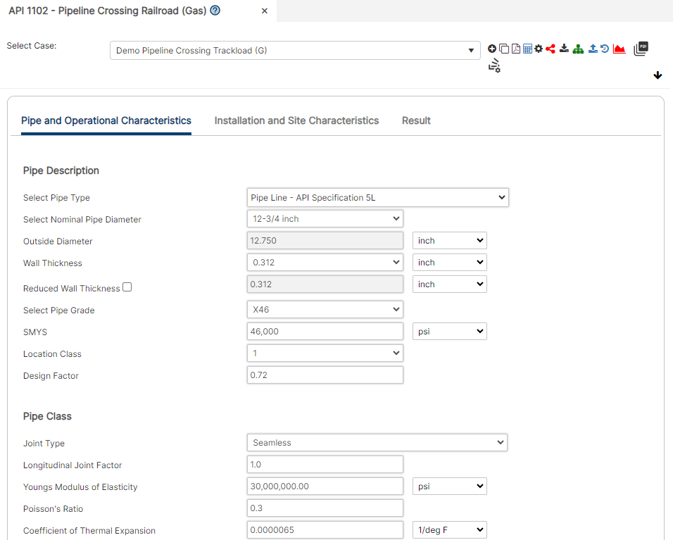
Pipe Properties
DIAMETER.
- The diameter, D, is the outside pipe diameter
- Has units of inches.
- The allowable range is from 2.000 to 42.000 in.
- The default value is D = 12.750 in.
MAXIMUM ALLOWABLE OPERATING PRESSURE.
- The maximum allowable operating pressure, MAOP, is used as the design internal pressure for calculating circumferential stress due to internal pressurization,
- Has units of psi,
- The allowable range is from 0 to 5,000 psig.
SPECIFIED MINIMUM YIELD STRENGTH.
- The specified minimum yield strength, SMYS,
- Has units of pounds per square inch (psi)
- Has a range of allowable values covering steel grades A25 (SMYS = 25000 psi) to X-80 (SMYS = 80000 psi).
- The SMYS is also used to establish the girth and longitudinal weld fatigue endurance limits.
DESIGN FACTOR, (F).
- Although 49 CFR 192 or 195, establishes a design factor, F, the user can input another F value.
- The allowable range is from 0.10 to 1.00.
- The default design factor is F = 0.72.
Allowable Total Stress Factor
- Governs the Allowable Effective Stress calculated in API 1102 calculation
- This is to allow overwriting design factor limitations when calculating Allowable Effective Stress.
- The default value is the design factor used. User has the option to overwrite this value to the recommended internal Standard Operating Procedure (SOP).
LONGITUDINAL JOINT FACTOR.
- The longitudinal joint factor, E, depends on the type of pipe welds.
- The input screen limits E to either 0.60, 0.80, or 1.00, consistent with the values given in 49CFR192, Section 192.113.
- The default value is E = 1.00.
INSTALLATION TEMPERATURE.
- The installation temperature, T1 is given in degrees Fahrenheit (°F).
- This value is used with T2 to determine thermal stress effects.
- The allowable range is from -20 to 450 °F.
OPERATING TEMPERATURE.
- The operating temperature, T2 is give in degrees Fahrenheit (°F).
- The T2 value is used to determine the temperature derating factor, T.
- T2 also is used with T1 to determine thermal stress effects.
- The allowable range is from -20 to 450 °F.
WALL THICKNESS.
- The pipe wall thickness, wt. has units of inches.
- The wall thickness to diameter ratios must be within the range of wt./D = 0.01 to 0.08.
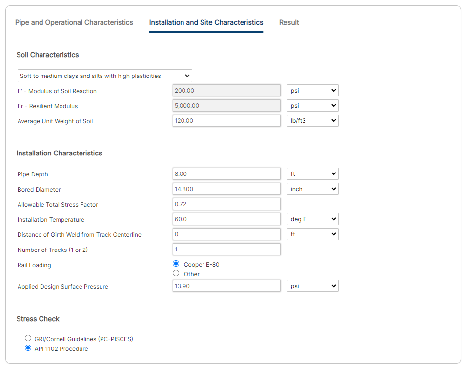
DEPTH OF CARRIER PIPE.
- The depth of the carrier pipe, H, is measured from the top of tie to the pipeline crown for railroads.
- Has units of feet (ft)
- Is used to establish the impact factor, Fi used in the design methodology.
- The allowable range for the live load design curves is from 6ft <= H <= 14 ft for railroads
BORED DIAMETER.
- The bored diameter, Bd (Bd in RP 1102), has units of inches.
- The minimum value is Bd = D, and the maximum value is Bd = D + 6 in.
- The default value is Bd = D + 2 in.
SOIL TYPE FOR THE EARTH LOAD
- The soil type for the earth load calculations is either A or B. See Figure 4 in API RP 1102.
MODULUS OF SOIL REACTION.
- The modulus of soil reaction, E’, has units of ksi.
- The minimum value allowed is E’ = 0.2 ksi, and the maximum input value for E’ is 8.0 ksi.
- The maximum recommended value for auger bored installations is E’ = 2.0 ksi.
- When an E’ value greater than 2.0 ksi is used, a warning will be displayed that the value is beyond the normal range of E’ for auger bored installations.
- See details in API RP 1102.
SOIL RESILIENT MODULUS.
- The soil resilient modulus, Er has units of ksi.
- The minimum allowable value for the live load design curves is Er = 5.00 ksi, and the maximum allowable value is Er = 20.0 ksi.
- See Table 3 in API RP 1102
- The default value is Er = 10.0 ksi, as recommended in API RP 1102.
SOIL UNIT WEIGHT.
- The soil unit weight, r, has units of pcf,
- The allowable range is from 0 to 150 pcf.
- The default value is r = 120 pcf.
TYPE OF LONGITUDINAL WELD
- The type of longitudinal weld is used with the SMYS to establish the longitudinal weld fatigue endurance limit, SFL.
- The choices for the type of longitudinal seam weld are SAW or ERW.
- See Table 3 in API RP 1102 for the influence of longitudinal weld type and SMYS on the seam weld fatigue endurance limits.
- The default type of longitudinal weld is SAW.
GIRTH WELD DISTANCE
- The girth weld distance, LG, is used to determine the longitudinal stress reduction factor, RF, needed for the girth weld fatigue calculations.
- has units of feet
- The allowable values range from 0 to 99 ft.
- When a double track crossing is being analyzed, the recommended value for LG is less than 5 ft.
- For LG less than 5 ft, longitudinal stress reduction factors are not used.
- See Figure 18 A and 18 B in API RP 1102 for the RF values as dependent on LG, H, and D.
NUMBERS OF TRACKS
- The number of tracks, Nt, is used to determine whether a single or double track railroad crossing will be analyzed.
- The Nt value determines the NH and NL factors for circumferential and longitudinal live load pipelines stresses, respectively.
- The default value is Nt = 1.
E-TYPE RAIL LOADING
- The E – Type rail loading is used to determine the applied surface stress, w, for railroad crossings.
- The allowable range is from 0 to 99.
- Can also be entered, which causes the surface load, w, to be 1.0 psi.
- The default value is E – 80 loading, as recommended in API RP 1102.
YOUNG’S MODULUS
- Young’s modulus of the steel carrier pipe, Es (Es in RP 1102), has units of ksi.
- The allowable values range from 29,000 to 31,000 ksi.
- The default value is Es = 30,000 ksi.
POSSION’S RATIO
- Possion’s ratio of the steel carrier pipe, s, is used to assess thermal and longitudinal stresses due to the circumferential earth load and internal pressure stresses.
- The allowable values range from 0.25 to 0.30.
- The default value is s = 0.30.
COEFFICIENT OF THERMAL EXPANSION.
- The coefficient of thermal expansion of the steel carrier pipe T, is given for temperature in °F, and is used to assess longitudinal thermal stresses.
- The range is from 0.0000060 to 0.0000080 per F.
- The default value is T = 0.0000065 per °F.
Workflow
Step 1: Check wall thickness for the operation pressure. To continue wt > wtd
wt_d=\frac{PD}{2S}FET
wt_d=\frac{PD}{2S}FETWhere:
wtd – Wall Thickness Minimum (in)
wt – Wall Thickness Actual (in)
D – Pipe Diameter (in)
S – Specified Minimum Yield Strength (psi)
P – Design Pressure (psi)
F – Design Factor
E – Longitudinal Joint Factor
T – Temperature Derating Factor
Step 2: Check Allowable Barlow Stress
SH_i=\frac{PD}{2wt}\~\SH_a=FET(S)
SH_i=\frac{PD}{2wt}\\~\\SH_a=FET(S)(see External Link: Barlow’s Formula in Wikipedia.com)
Step 3: Circumferential stress due to Earth Load
Soil type – Default Value: (Kμ= 0.165 for Soil Type A, Kμ= 0.192 for Soil Type B)
\frac{H}{B_d},\frac{B_d}{D},\frac{wt}{D}
\frac{H}{B_d},\frac{B_d}{D},\frac{wt}{D}Where:
𝐻 − Pipe Depth (ft)
𝐵𝑑 − Bored Diameter (in)
𝐸𝑝𝑟𝑖𝑚𝑒 − Modulus of Soil Reaction
𝐸𝑟 − Resilient Module
𝛾 − Average unit weight of soil
𝐸𝑠 − Young′s Modulus of Elasticity
\text{numerator} = 0.507E_s \left( \frac{wt}{D} \right) + 0.006E_{prime} (1000) \left( \frac{D}{wt} \right) \left( \frac{D}{wt} \right)\~\ \text{denominator} = E_s \left( \frac{wt}{D} \right) \left( \frac{wt}{D} \right) \left( \frac{wt}{D} \right) + 0.915E_ \text{prime} (1000)
\text{numerator} = 0.507E_s \left( \frac{wt}{D} \right) + 0.006E_{prime} (1000) \left( \frac{D}{wt} \right) \left( \frac{D}{wt} \right)\\~\\ \text{denominator} = E_s \left( \frac{wt}{D} \right) \left( \frac{wt}{D} \right) \left( \frac{wt}{D} \right) + 0.915E_ \text{prime} (1000)
Where:
\begin{align} & \text{Part 1 Reference:} = \frac{\text{numerator}}{\text{denominator}}\~\ & \text{Part 2 Reference:} = \left(\frac{1 – e^{-2(K_\mu)\left( \frac{h}{B_d} \right)}}{2(K_\mu)}\right)\~\ & \text{Part 3 Reference:} = \left( \frac{B_d}{D} \right)^2 \~\ & KH_e = (\text{Part 1}) (\text{Part 2}) (\text{Part 3}) \end{align}
\begin{align*}
& \text{Part 1 Reference:} = \frac{\text{numerator}}{\text{denominator}}\\~\\
& \text{Part 2 Reference:} = \left(\frac{1 - e^{-2(K_\mu)\left( \frac{h}{B_d} \right)}}{2(K_\mu)}\right)\\~\\
& \text{Part 3 Reference:} = \left( \frac{B_d}{D} \right)^2 \\~\\
& KH_e = (\text{Part 1}) (\text{Part 2}) (\text{Part 3})
\end{align*}
\frac{H}{B_d} = \frac{(H)(12)}{B_d} \~\
B_e =\frac{ \left(\frac{1 – e^{-2(K_{\mu})\left(\frac{h{(12)}}{B_d}\right)})}{2(K_{\mu})}\right)}{ \quad (\text{Part 2 Ref})} \~\
E_e = \frac{\left( \frac{B_d(12)}{D} \right) \left( \frac{B_d(12)}{D} \right)} {(\text{Part 3 Ref})} \~\
\frac{\gamma}{pci} = \frac{\gamma}{1728} \~\
SH_e = KH_eB_eE_e \frac{\gamma}{pci} D
 \frac{H}{B_d} = \frac{(H)(12)}{B_d} \\~\\
 B_e =\frac{ \left(\frac{1 - e^{-2(K_{\mu})\left(\frac{h{(12)}}{B_d}\right)})}{2(K_{\mu})}\right)}{ \quad (\text{Part 2 Ref})} \\~\\
 E_e = \frac{\left( \frac{B_d(12)}{D} \right) \left( \frac{B_d(12)}{D} \right)} {(\text{Part 3 Ref})} \\~\\
 \frac{\gamma}{pci} = \frac{\gamma}{1728} \\~\\
 SH_e = KH_eB_eE_e \frac{\gamma}{pci} D
Step 4: Impact Factor and Applied Design Surface Pressure
(F-Flexible, R-Rigid, N-None) (Case 1,2,3) Determine the Critical Load case and the applied surface design load. Find these values from Table Impact Factor:
\text{If Depth of Cover} \leq 5\text{ft}, 1.75,= {(1.75 – 0.03)(\text{Cover} – 5)} \~\NH=(0.825+0.0375H)+\left( \frac{0.2}{42}\right)D
\text{If Depth of Cover} \leq 5\text{ft}, 1.75,= {(1.75 - 0.03)(\text{Cover} - 5)} \\~\\NH=(0.825+0.0375H)+\left( \frac{0.2}{42}\right)D
Where:
NH – Railroad Double Track Factor for Circumferential Stress
NL – Railroad Double Track Factor for Longitudinal Stress
Step 5: Cyclic Stress, 𝑫𝑺𝑯𝒉 & 𝑫𝑺𝑳𝒉
Reference the Design Curves in Appendix A from “Technical Summary and Database for Guidelines for Pipelines Crossing Beneath Railroads and Highways” (GRI-91/0285, Final Report)
Where:
𝐾𝐻𝑟 − Railroad Stiffness Factor for Cyclic Circumferential Stress
𝐺𝐻𝑟 − Railroad Geometry Factor for Cyclic Circumferential Stress
𝐷𝑆𝐻𝑟 − Cyclic Circumferential Stress
𝐾𝐿𝑟 − Railroad Stiffness Factor for Cyclic Longitudinal Stress
𝐺𝐿𝑟 − Railroad Geometry Factor for Cyclic Longitudinal Stress
𝐷𝑆𝐿𝑟 − Cyclic Longitudinal Stress
Step 6: Circumferential Stress due to Internal Pressurization Shi
SH_i=\frac{P(D-wt)}{2wt}
SH_i=\frac{P(D-wt)}{2wt}Step 7: Principle Stresses 𝑺𝟏,𝑺𝟐,𝑺𝟑
Where:
\begin{align} &S_1 = SH_e + DSH_h + SH_i &\~\ &S_2 = DSL_h – E_s(1000) \alpha t(T_2 – T_1) + ns(SH_e + SH_i)&\~\ &S_3 = -P&\~\ &S_{eff} = \sqrt{0.5((S_1 – S_2)^2 + (S_2 – S_3)^2 + (S_3 – S_1)^2)}& \end{align}
\begin{align*} &S_1 = SH_e + DSH_h + SH_i &\\~\\ &S_2 = DSL_h - E_s(1000) \alpha t(T_2 - T_1) + ns(SH_e + SH_i)&\\~\\ &S_3 = -P&\\~\\ &S_{eff} = \sqrt{0.5((S_1 - S_2)^2 + (S_2 - S_3)^2 + (S_3 - S_1)^2)}& \end{align*}Case Guide
Part 1: Create Case
- Select the API 1102 Gas Pipeline Crossing – Railroad application from the Pipeline Crossing module
- To create a new case, click the “Add Case” button
- Enter Case Name, Location, Date and any necessary notes.
- Fill out all required Parameters.
- Make sure the values you are inputting are in the correct units.
- Click the CALCULATE button to overview results.
Input Parameters
- Pipe Type
- Nominal Pipe Size(in):(1/8” – 48”)
- Pipe Outside Diameter(in):(0.625” – 48”)
- Pipe Wall Thickness(in):(0.068”- >2”)
- Young’s Modulus of Elasticity:(29000000psi – 30000000psi)
- Poisson’s Ratio (-1 – 0.5)
- Thermal Expansion Coefficient(1/°F) :(0.0000022in/inF – 0.000012in/inF)
- Joint Type
- Location Class: Refer 49 CFR 192.5
- Operating Pressure
- Operating Temperature
- Specified Minimum Yield Stress:(24000psi-80000psi)
- Design Factor: Reference 49 CFR 192.611
- Longitudinal Joint Factor
- Temperature Derating Factor
- Modulus of Soil Reaction
- Resilient Modulus
- Average unit weight of Soil:(70lb/ft3 – 150lb/ft3)
- Pipe Depth
- Bored Diameter
- Installation Temperature
- Distance of Girth Weld from Track Centerline
- Number of Tracks
- Rail Loading
- Applied Design surface Pressure
- Safety Factor for Effective Stress
- Safety Factor for Girth Welds
- Safety Factor for Longitudinal Welds
Part 2: Outputs/Reports
- If you need to modify an input parameter, click the CALCULATE button after the change.
- To SAVE, fill out all required case details then click the SAVE button.
- To rename an existing file, click the SAVE As button. Provide all case info then click SAVE.
- To generate a REPORT, click the REPORT button.
- The user may export the Case/Report by clicking the Export to Excel icon.
- To delete a case, click the DELETE icon near the top of the widget.
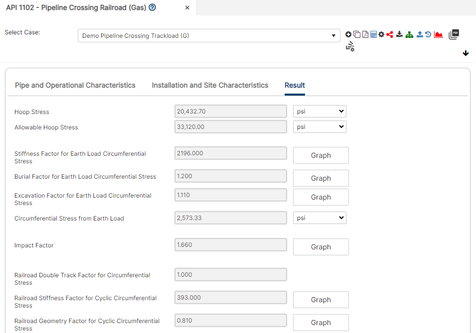
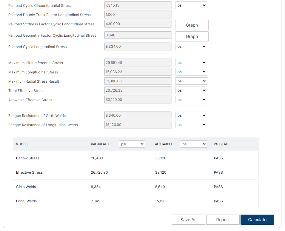
Results
- Hoop Stress
- Allowable Hoop Stress
- Stiffness Factor for Earth Load Circumferential Stress
- Burial Factor for Earth Load Circumferential Stress
- Excavation Factor for Earth Load Circumferential Stress
- Circumferential Stress from Earth Load
- Impact Factor
- Railroad Double Track Factor for Circumferential Stress
- Railroad Stiffness Factor for Cyclic Circumferential Stress
- Railroad Geometry Factor for Cyclic Circumferential Stress
- Railroad Cyclic Circumferential Stress
- Railroad Double track factor for Longitudinal Stress
- Railroad Stiffness Factor for Cyclic Longitudinal Stress
- Railroad Geometry Factor for Cyclic Longitudinal Stress
- Railroad Cyclic Longitudinal Stress
- Maximum Circumferential Stress
- Maximum Longitudinal Stress
- Maximum Radial Stress
- Total Effective Stress
- Allowable Effective Stress
- Fatigue Resistance of Girth Welds
- Fatigue Resistance of Longitudinal Welds
- Barlow Stress
- Effective Stress
- Girth Welds
- Long Welds
Reference
- Battelle Petroleum Technology Report on “Evaluation of Buried Pipe Encroachments” which considered the theoretical work done by M.G. Spangler on overburden and vehicle loads on buried pipe.
- “Technical Summary and Database for Guidelines for Pipelines Crossing Beneath Railroads and Highways” (GRI-91/0285, Final Report)
- Cornell/GRI Guidelines are given in “Guidelines for Pipelines Crossing Beneath Highways” (Stewart, et al., 1991b) and “Guidelines for Pipelines Crossing Beneath Highways”.
- ASME B31.8 “Gas Transmission and Distribution Systems” “Evaluation of Buried Pipe Encroachments”, BATTELLE, Petroleum Technology Center, 1983
- API RP 1102 – Steel Pipelines Crossing Railroads and Highways
FAQ
-
What are crossings – Live Load?
Many questions are asked about API 1102 regarding wheel load cyclic stresses on highways and railroads.
Live highway load, w, the load due to the wheel load at the highway surface. The load from only one wheel set needs to be considered. An axle is considered to have two-wheel sets.
Live rail load, w, pounds per sq inch, is the load applied at the surface of the crossing. It is assumed that the load is evenly distributed over an area that is 8’x 20’.The recommended default is 80,000 pounds (80 Kips) per axle. Check Out
-
Validation checks in place for API 1102 – Pipeline Crossing Railroad?
Below are the list of validation checks we have incorporated in API 1102 – Pipeline Crossing Railroad (Gas and Liquid). Check Out
-
Validation checks in place for API 1102 – Pipeline Crossing Highway?
Below are the list of validation checks we have incorporated in API 1102 – Pipeline Crossing Highway (Gas and Liquid). Check Out
-
Track Load – Interpolation Method (for Influence Coefficient)?
We recently issued an enhancement for Track load calculation by providing an option to use the Interpolation Method to calculate the Influence Coefficient (Ic). The old method calculated the Influence Coefficient using a roundoff method for ‘m-Influence Factor’ and ‘n-Influence Factor’ to get the Influence Coefficient from the table. Check Out
-
API 1102 Uncased Crossing 10 Foot Limit Understanding?
Uncased carrier pipe is subjected to internal loading from pressure and external loading from earth loading (dead load) and live (cyclic) loading from highway or railroad traffic. Other loading due to special or temporary conditions should be evaluated on the specific situation in the field (See Knowledge Base Article for Temporary Conditions). Check Out
-
Surface Load Mitigation Measures – Best Practice?
Method
Reduce the operating pressure of the pipeline.
Advantages
Provides a direct reduction of the hoop stress due to internal pressure. This reduction allows for additional circumferential stress due to equipment loads.
Disadvantages
– Reduces the beneficial effect of internal pressure on the pipe circumferential bending stresses due to fill and traffic loads.
– Could reduce the overall capacity of the pipeline and therefore should not be considered as a long term fix.
-
Difference between “Operating Weight” in Track Load Analysis and “concentrated surface load” in Wheel Load?
The term “Operating Weight” used in the track load analysis is a straight forward analysis as it takes the total weight of the equipment into consideration. We multiply the total weight by 0.5 to reflect the load on each track (see below the equation).
“Concentrated surface load” in the Wheel load calculation requires a more detailed understanding of the vehicle that is crossing. Below schematic will help better understand the requirement for “Concentrated surface load” entry in Wheel Load analysis.
-
Determining Trench Width for Crossings?
The basic analysis developed by M.G. Spangler includes frictional forces between the trench wall and the backfill. This permits the weight of the overburden to be partially carried by the surrounding soil and reduces the total soil load on the pipe. The equations require the following information to determine internal friction. Check Out
-
Combined Stress for Wheel Load and Track Load?
The question comes up from time to time how to address local stresses for wheel and track load calculations. ASME B31.8 833.9 Local Stresses states that the maximum allowable sum of circumferential stress due to internal pressure (Barlow Design Formula) and circumferential through-wall bending stress caused by surface vehicle loads or other local loads is 0.9ST, where S is the specified minimum yield strength, psi (MPA) per para. 841.1 (a), and T is the temperature derating factor per para. 841.1.8. Check Out
-
What Are Timber Mats in Crossing?
Timber mats are used for temporary access roads, work pads, staging areas, and to stabilize the ground beneath heavy equipment, dissipating heavy loads and providing equipment stability.
For short-term water crossings over narrow spans timber mats (also referred to as bridge mats) or crane mats may be an option.
For projects that require moving heavy equipment safely across pipelines, timber mats can be used to create air bridges which will support the weight of heavy equipment while protecting the pipelines below. Air bridges can also be used to cross culverts, ditches, or sensitive ground that needs to be bridged. Check Out
-
Redistributing Wheel and Track Loads (Pavement and Other Materials)?
This knowledge base article is a takeoff from “Pipeline Toolbox (PLTB) and Vehicles over Buried Pipelines – Maximum Allowable Stress”. These predictions through Spangler’s work, Battelle and others who contributed to validation makes PLTB one of most used programs in the industry. It includes temporary wheel and track load crossings that considers a uniformly distributed load at the surface while calculating the load on the pipe. This article will focus on concrete, asphalt and timber mats as well as other materials such as steel plates and composites. The other materials are not part of the Pipeline Toolbox which will be discussed. Check Out
-
Pipeline Crossings – External Loads and Vehicles over Buried Pipelines “Maximum Allowable Combined Stress”?
This article was created due to the number of inquiries regarding the Maximum Allowable Combined Stress for Class 3 Design Areas. The research by M. G. Spangler, Battelle and industry allowed this information to be a standard practice today with Wheel and Track Load analysis today. Check Out
-
Applicability of Class Location for Liquid Lines? What is the design factor used for Liquid Pipeline Operation?
Design factor specification for Liquid Pipelines are governed by ASME B31.4 Table 402.3.1(a)
Excerpts from B31.4: Check Out
-
Loading Requirements for API 1102 E-80 and E-90 Railroad Crossings?
API 1102 for railroad crossing program is based on the design methodology that has been used in analyzing existing uncased pipelines and designing new uncased pipelines that cross beneath railroads. This API design methodology relates to the train engine (E-80) which is the heaviest load: Check Out
-
What are Cased Crossings?
The pipeline industry begins to experience casing problems such as carrier pipe leaks/failures under road crossings.
- Atmospheric corrosion due to condensation (particularly at elevated temperatures and cold soils)
- Metal to metal shorts
- Electrolytic coupling or contact
Can the casing pipe protect the carrier pipe from external loadings? Check Out
-
Understanding Impact Factors in Pipeline Design (CEPA)
What is an Impact Factor?
An impact factor is a multiplier used in pipeline design to account for the additional stress caused by moving vehicles above the pipeline, compared to static loads. Think of it as a “safety buffer” that accounts for the dynamic nature of traffic. Check Out