API 1104 Weld Imperfection Assessment – Liquid

Determination of Acceptable imperfection Size by Option 1

Two sets of acceptance criteria are given, depending on the CTOD toughness value.

When the CTOD toughness is equal to or greater than 0.010 in. (0.25 mm), the maximum acceptable imperfection size is given in Figure A.7 at various load levels (P_r). If the load level is not given in Figure A.7, the maximum acceptable imperfection size can be obtained by interpolating the adjacent curves or by taking the value of the next higher load level.

When the CTOD toughness is equal to or greater than 0.004 in. (0.10 mm) and less than 0.010 in. (0.25 mm), the maximum acceptable imperfection size is given in Figure A.8.

The acceptable imperfection size may be more limiting than that from the Option 2 procedure as the limits in Figure A.7 and Figure A.8 were calibrated to a CTOD toughness of 0.010 in. (0.25 mm) and 0.004 in. (0.10 mm), respectively.

The total imperfection length shall be no greater than 12.5% of the pipe circumference. The maximum imperfection height shall be no greater than 50% of the pipe wall thickness.

The allowable height of the buried imperfections is treated the same as the allowable height of the surface-breaking imperfections.

The built-in safety factor in the acceptable imperfection size can accommodate certain amount of under sizing of imperfection height without negatively impacting weld integrity. The assumed height uncertainty is the lesser of 0.060 in. (1.5 mm) and 8% of pipe wall thickness. No reduction in allowable imperfection size is necessary if the allowance for inspection (alternatively termed inspection error) is better than the assumed height uncertainty.

The allowable imperfection height shall be reduced by the difference between the allowance for inspection and the assumed height uncertainty if the above condition cannot be met.

Step 1. Determine Flow Stress

It is necessary to determine material’s flow stress in order to obtain the load level P_r. The flow stress is the averaged value of the SMYS and SMTS. Alternatively, the flow stress of API 5L Grade X52 to X80 may be conservatively estimated as: \sigma_f=\sigma_y\bigg[ 1+\bigg( \frac{21.75}{\sigma_y} \bigg)^{2.30}\bigg]

\sigma_f=\sigma_y\bigg[ 1+\bigg( \frac{21.75}{\sigma_y} \bigg)^{2.30}\bigg]

Where:
𝜎_𝑓 − Flow Stress (ksi)
𝜎_𝑦 − Pipe Grade (ksi)
𝜎_𝑎 − Axial Design Stress (ksi)

Step 2. Determine Applied Load Level

P_r=\frac{\sigma_a}{\sigma_f}

P_r=\frac{\sigma_a}{\sigma_f}

Step 3. Determine Initial Allowable Imperfection Size

Figure A.7 is utilized for determining the initial allowable imperfection size (CTOD ≥ 0.010 in. or 0.25 mm). The curve of P_r = 0.825 in the figure is now used for the interpolations. The allowable imperfection size is tabulated in Table A.2 and shown in Figure A.9.

Step 4. Determine Height Adjustment

Assumed height uncertainty = lesser of 8% WT and 0.060 in. = 0.040 in. (1.02 mm).
Allowance for inspection (i.e. inspection error) = 0.050 in. (1.27 mm).
Imperfect height adjustment = Allowance for inspection – Assumed height uncertainty
= 0.050 – 0.040
= 0.010 in. (0.25 mm)

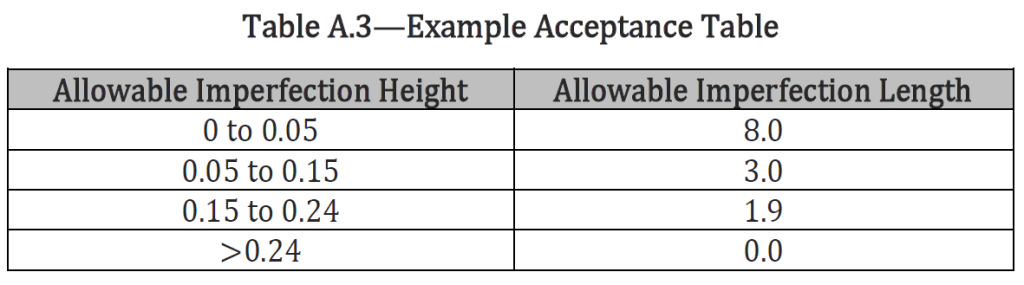
Step 5. Produce Final Acceptance Table

The results of the ECA should be tabulated in a user-friendly format. Table A.3 suggests an operator-friendly format for this ECA example. However, a project with a heavier wall thickness may have more rows in a similar table.

Determination of Acceptable Imperfection Size by option 2

Background

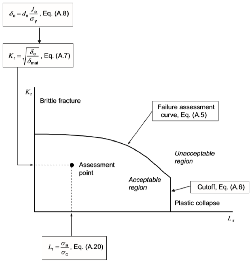
The underlining Option 2 procedure is the FAD. There are three key components in the assessment in FAD format, see Figure A.10:

1. Failure Assessment Curve (FAC);
2. Stress or Load Ratio, S_r or L_r; and
3. Toughness Ratio, k_r

The FAC is a locus that defines the critical states in terms of the stress and toughness ratios. The stress ratio defines the likelihood of plastic collapse. The toughness ratio is the ratio of applied crack driving force over the material’s fracture toughness. It defines the likelihood of brittle fracture.

The FAD approach is computationally complex. Proficiency and understanding of fracture mechanics are necessary to ensure the procedure is applied correctly. A validated computer program should greatly simplify the computation.

Determination of Critical Imperfection Size

The critical imperfection size can be computed iteratively using equations provided in the equation below. The following steps may be followed. : K_r = f(L_r) = (1 – 0.14L_r^2)\left[0.3 + 0.7\exp(-0.65L_r^6)\right]

K_r = f(L_r) = (1 - 0.14L_r^2)\left[0.3 + 0.7\exp(-0.65L_r^6)\right]

Where:
𝐾_𝑟 − Toughness Ratio
𝐿_𝑟 − Stress Ratio

The cut-off of the FAC on the L_r axis is at: L^{cuttoff}r=\sigma_f\Delta\sigma_y

L^{cuttoff}r=\sigma_f\Delta\sigma_y

Where the flow stress σ_f is the averaged value of SMYS and SMTS, or alternatively determined by Equation (A.3).

Step 1. Select an imperfection size as a start point. A reasonable start point is an imperfection with the maximum allowed height, η = 0.5, and a small imperfection length that represents the smallest imperfection length that the selected inspection methods can confidently detect.

Step 2. Determine the assessment point in the FAD format in accordance with A.5.1.4.3.

Step 3. If the assessment point falls inside the safe region, increase the imperfection length and repeat Step 2

Step 4. If the assessment point falls outside the safe region, decrease the imperfection length and repeat Step 2.

Step 5.If the assessment point falls on the FAC:

• This represents a critical state with the combination of load, material property, and imperfection size. Make a note of the imperfection height and length.
• Reduce the imperfection height by a small increment, say Δη = 0.05. Start from the imperfection length determined in Item a) and repeat Step 2).

Step 6. Make a table of critical imperfection height and length.

Step 7. Apply a safety factor of 1.5 on the imperfection length to produce a draft table of the allowable imperfection height versus imperfection length.

Step 8. Make necessary adjustment to the draft table to ensure detectability of the selected inspection methods and sound welding practice. Produce the final table of the allowable imperfection height versus imperfection length.

The total imperfection length shall be no greater than 12.5 % of the pipe circumference. The maximum imperfection height shall be no greater than 50 % of the pipe wall thickness.

The allowable height of the buried imperfections is treated the same as the allowable height of the surface-breaking imperfections.

The built-in safety factor in the acceptable imperfection size can accommodate certain amount of under sizing of imperfection height without negatively impacting weld integrity. The assumed height uncertainty is the lesser of 0.060 in. (1.5 mm) and 8% of pipe wall thickness. No reduction in allowable imperfection size is necessary if the allowance for inspection is better than the assumed height uncertainty.

The allowable imperfection height shall be reduced by the difference between the allowance for inspection and the assumed height uncertainty if the above condition cannot be met.

Assessment Point, Toughness Ratio K_r

K_r=\sqrt{\frac{\delta_e}{\delta_{mat}}}

K_r=\sqrt{\frac{\delta_e}{\delta_{mat}}}

Where:
𝐾_𝑟 − Toughness Ratio
𝛿_𝑚𝑎𝑡 − CTOD Toughness of Material
𝛿_𝑒 − CTOD Driving Force

\delta_e = d_n \frac{J_e}{\sigma_y}

\delta_e = d_n \frac{J_e}{\sigma_y}

𝐽_𝑒 − Elastic part of J Integral (ksi)
𝜎_𝑦 − Specified Minimum Yield Strength of Pipe Material, SMYS (ksi)

d_n = 3.69 \left(\frac{1}{n}\right)^2 – 3.19 \left(\frac{1}{n}\right) + 0.882

d_n = 3.69 \left(\frac{1}{n}\right)^2 - 3.19 \left(\frac{1}{n}\right) + 0.882

𝑑_𝑛 − J Integral to COTD Conversion Factor
𝑛 − Strain Hardening Exponent

\varepsilon = \frac{\sigma}{E} + \left(0.005 – \frac{\sigma_y}{E}\right) \left(\frac{\sigma}{\sigma_y}\right)^n

\varepsilon = \frac{\sigma}{E} + \left(0.005 - \frac{\sigma_y}{E}\right) \left(\frac{\sigma}{\sigma_y}\right)^n

𝜀 − Strain
𝜎 − Stress
𝑛 − Strain Hardening Exponent
𝐸 − Young′s Modulus of Elasticity (psi)

The strain hardening exponent may be estimated from Y/T ratio: n = \frac{\ln(\varepsilon_t / 0.005)}{\ln {1 / (Y / T)}}

n = \frac{\ln(\varepsilon_t / 0.005)}{\ln \{1 / (Y / T)\}}

For ferritic material of API 5L Grades X52 to X80, the Y/T ratio may be estimated as: Y/T=\frac{1}{1+2\bigg(\frac{21.75}{\sigma_y} \bigg)^{2.30}}

Y/T=\frac{1}{1+2\bigg(\frac{21.75}{\sigma_y}  \bigg)^{2.30}}

and the uniform strain is estimated as: \varepsilon=-0.00175\sigma_y+0.22

\varepsilon=-0.00175\sigma_y+0.22

The elastic J integral is given as: J_e = \frac{K_1^2}{E/(1 – \nu^2)}\~\K_l = \sigma_a \sqrt{\pi a F_b}

J_e = \frac{K_1^2}{E/(1 - \nu^2)}\\~\\K_l = \sigma_a \sqrt{\pi a F_b}

𝐾_𝑙 − Stress Intensity Factor (ksi)
𝐹_𝑏 − is a function of pipe diameter ratio,𝛼,and relative imperfection length,𝛽,and relative imperfection height 𝜂:

F_b(\alpha, \beta, n) =
\begin{cases}
F_{b0}(\alpha, \beta, n) & n \geq 0.1 \text{ and } \beta \leq \frac{80}{\pi}\frac{n}{\alpha} \
F_{b0} \left( \alpha, \beta= \frac{80}{\pi}\frac{n}{\alpha},n \right) & n \geq 0.1 \text{ and } \beta>\frac{80}{\pi}\frac{n}{\alpha} \
F_{b0} \left( \alpha, \beta=\frac{80}{\pi}\frac{ 0.1}{\alpha},0.1 \right) & n < 0.1
\end{cases}

F_b(\alpha, \beta, n) = 
\begin{cases} 
F_{b0}(\alpha, \beta, n) &  n \geq 0.1 \text{ and } \beta \leq \frac{80}{\pi}\frac{n}{\alpha} \\
F_{b0} \left( \alpha, \beta= \frac{80}{\pi}\frac{n}{\alpha},n \right) &  n \geq 0.1 \text{ and } \beta>\frac{80}{\pi}\frac{n}{\alpha} \\
F_{b0} \left( \alpha, \beta=\frac{80}{\pi}\frac{  0.1}{\alpha},0.1 \right) &  n < 0.1
\end{cases}

Where: F_b(\alpha, \beta, n) = \bigg( 1.08 + 2.31 \alpha^{0.791} \beta^{0.906} n^{0.983} \frac{m_1}{\alpha \beta}+{\alpha^{0.806} \beta m_2} \bigg)

F_b(\alpha, \beta, n) = \bigg( 1.08 + 2.31 \alpha^{0.791} \beta^{0.906} n^{0.983} \frac{m_1}{\alpha \beta}+{\alpha^{0.806} \beta m_2} \bigg)

𝑚₁ = −0.00985 − 0.163𝑛 − 0.345𝑛²
𝑚₂ = −0.00416 − 2.18𝑛 − 0.155𝑛²

Case Guide

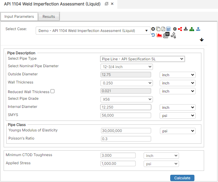
Part 1: Create Case

Input Parameters

• Nominal Pipe Size (in): (0.625” – 48”)
• Wall Thickness (in): (0.068”- >2”)
• Pipe grade: (24000psi-80000psi) (if unknown use Grade A 24000), Minimum CTOD Toughness (in)
• Young’s Modulus of Elasticity (psi)
• Poisson’s Ratio
• Minimum CTOD Toughness (in)
• Applied Stress (psi)

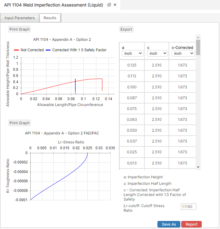
Part 2: Outputs/Reports

Results

• Allowable Height/Pipe Wall Thickness
• Allowable Length/Pipe Circumference
• K – Toughness Ratio

References

• Pipeline Design for Hydrocarbons Gases and Liquids, Committee of pipeline planning, American Association of Civil Engineers, 1975
• Engineering Data Book, Volume II, Gas Processor Association, Revised Tenth Edition, 1994
• Pipeline Design & Construction, A Practical Approach, American Society of Mechanical Engineers, 2000

FAQ