
Introduction
The Track Load Program was designed to calculate the overburden and track loads on buried pipe with a Single Layer System (soil only). The information used to design this program was taken from the Newmark’s Integration of the Boussinesq Equation which considered the theoretical work done by M.G. Spangler on overburden and vehicle loads on buried pipe. This analysis does not evaluate cyclic loading, but the API 1102 calculation does.
Variables and Boundary Conditions
REQUIRED INFORMATION:
- Values for all the following variables:
- 𝐻2 −Cover, Vertical Depth from the Ground to the Top of the Pipe (ft.)
- 𝐵 − Trench Width (ft.)
- 𝐷𝑠 − Weight per unit Volume of Backfill (lbs/ft3)
- 𝐷 − Outside Diameter of the Pipe (in.)
- 𝑆𝑀𝑌𝑆 − Specified Minimum Yield Stress of the Pipe (psi.)
- 𝑃 − Pipe Internal Pressure (psi.)
- 𝑇 − Pipe Wall Thickness (in.)
- Variables for the following information about the track:
- 𝐿𝑡 − Operating Weight of the Object Crossing the Pipeline with Tracks(lbs)
- 𝑇𝑤 − Width of the Standard Track Shoe(in)
- 𝑇𝑙 − Length of the Track on the Ground(ft)
- 𝑇𝑔 − Track Gauge(ft)
- The Design Factor of the pipeline being analyzed is used to find the Maximum Allowable Combined Stress (% SMYS), (0.72 is the standard factor used for liquid).
- The Soil Type which is used to find the friction force coefficients (Km), see Table II.
- The Crossing Construction Type which is used to find the bedding constants for buried pipe (Kb & Kz), see Table V & Figure 3.
- All the above information along with values for the following variables:
- X – Longitudinal Distance over which Deflection Occurs (ft)
- Y – Vertical Deflection (in)
Workflow
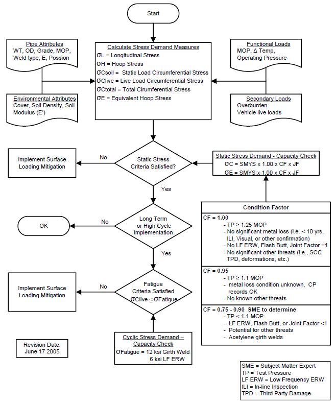
Pipeline Surface Load Acceptability Process:
The pressure exerted on the pipe at pipeline depth due to a load at the surface can be calculated using Boussinesq’s equation:
(1)
P_{\text{live}} = \frac{W_{\text{live}}}{D} = \frac{3 \cdot F}{2 \pi H^2 \left[1 + \left(\frac{d}{H}\right)^{2}\right]^{2.5}}
P_{\text{live}} = \frac{W_{\text{live}}}{D} = \frac{3 \cdot F}{2 \pi H^2 \left[1 + \left(\frac{d}{H}\right)^{2}\right]^{2.5}}
Where:
- Plive = Pressure on the pipe due to the live load (psi)
- Wlive = Live load on the pipe (lb/in)
- D = Diameter of the pipe (in)
- F = Point load at the surface (lb)
- H = Depth of soil cover (in)
- d = Offset distance from the pipe to the line of application of the surface load (in)
Using this equation, a tire, track, or any other load with a known contact area can be represented by a series of point loads at the surface, and the total load on the pipe is calculated as the summation of the effect of the individual loads.
The CEPA equation combines the pressure stiffening and soil restraint terms into a single equation for determining circumferential (hoop) bending stresses due to live or soil loads:
(2)
\sigma_{H_live} = \frac{3 \cdot K_b \cdot P_{\text{live}}\cdot \left(\frac{D}{t}\right)^2}{1 + 3 \cdot K_z\cdot \frac{P}{E} \cdot\left(\frac{D}{t}\right)^3 + 0.0915 \cdot \frac{E’}{E}\cdot \left(\frac{D}{t}\right)^3}
\sigma_{H\_live} = \frac{3 \cdot K_b \cdot P_{\text{live}}\cdot \left(\frac{D}{t}\right)^2}{1 + 3 \cdot K_z\cdot \frac{P}{E} \cdot\left(\frac{D}{t}\right)^3 + 0.0915 \cdot \frac{E'}{E}\cdot \left(\frac{D}{t}\right)^3}
Where:
- σH_live= circumferential (hoop) bending stress due to the live load (psi)
- Kb = Soil parameter
- t = Wall thickness (in)
- Kz = Soil parameter
- P = Internal pressure (psig)
- E = Young’s modulus of elasticity for steel (30×106 psi)
- E’ = Modulus of soil reaction (psi)
and
(3)
\sigma_{H_soil} = \frac{3 \cdot K_b \cdot P_{\text{soil}}\cdot \left(\frac{D}{t}\right)^2}{1 + 3 \cdot K_z\cdot \frac{P}{E} \cdot\left(\frac{D}{t}\right)^3 + 0.0915 \cdot \frac{E’}{E}\cdot \left(\frac{D}{t}\right)^3}
\sigma_{H\_soil} = \frac{3 \cdot K_b \cdot P_{\text{soil}}\cdot \left(\frac{D}{t}\right)^2}{1 + 3 \cdot K_z\cdot \frac{P}{E} \cdot\left(\frac{D}{t}\right)^3 + 0.0915 \cdot \frac{E'}{E}\cdot \left(\frac{D}{t}\right)^3}Where:
- σH_soil = Circumferential (hoop) bending stress due to the soil load (psi)
The circumferential (hoop) stress due to internal pressure is given as:
(4)
\sigma_{H_internal}=\frac{P\cdot D}{2\cdot t}
\sigma_{H\_internal}=\frac{P\cdot D}{2\cdot t}Where:
- σH_internal = Circumferential (hoop) stress due to internal pressure (psi)
The total circumferential stress, , is the sum of the stresses due to circumferential bending along with the hoop stress due to internal pressure. The total circumferential stress is compared to the allowable limit.
Internal pressure in pipelines restrained in soil causes a longitudinal stress equal to:
(5)
\sigma_{L_internal}=v\cdot\sigma_{H_internal}
\sigma_{L\_internal}=v\cdot\sigma_{H\_internal}Where:
- σL_internal = Longitudinal stress due to internal pressure (psi)
- v = Poisson’s ratio for steel (0.3)
In a manner similar to the longitudinal stress from pressure, the soil load causes a longitudinal stress equal to:
(6)
\sigma_{L_soil}=v\cdot\sigma_{H_soil}
\sigma_{L\_soil}=v\cdot\sigma_{H\_soil}Where:
- σL_soil = Longitudinal stress due to soil load (psi)
The longitudinal stress due to the live load is determined as a combination of stress due to local bending and beam deflection. The calculation for the local longitudinal stress caused by the surface load is estimated using Bjilaard’s solutions for local loading on a pipe found in Roark’s Formulas for Stress and Strain.
(7)
\sigma_{L_{local}} = \frac{0.153}{1.56} \cdot \beta^{4} \cdot \sigma_{H_{live}}
\sigma_{L\_{local}} = \frac{0.153}{1.56} \cdot \beta^{4} \cdot \sigma_{H\_{live}}
Where:
- σL_local = local bending stress (psi)
and
(8)
\beta = \left[12 \cdot (1 – v^{2})\right]^{1/8}
\beta = \left[12 \cdot (1 - v^{2})\right]^{1/8}
The vehicle load causes an axial pipeline deflection, which adds to the longitudinal stress due to internal pressure and temperature differential. If the pipeline is modeled as a beam on an elastic foundation, the maximum bending moment is given by Hetenyi1 as:
(9)
M = \frac{P_{\text{pipe}} \cdot D}{4\lambda^2} (2e^{-\lambda x} \sin \lambda x)
M = \frac{P_{\text{pipe}} \cdot D}{4\lambda^2} (2e^{-\lambda x} \sin \lambda x)
Where:
- M = Bending moment (in-lb)
- Ppipe = Pressure on pipe from an equivalent point load (psi)
- λ = Characteristic length (in-1)
- x = Distance along the pipeline (in)
and
(10)
\lambda = \sqrt[4]{\frac{E’ \cdot D \cdot \theta}{4 \cdot E \cdot I}}
\lambda = \sqrt[4]{\frac{E' \cdot D \cdot \theta}{4 \cdot E \cdot I}}
Where:
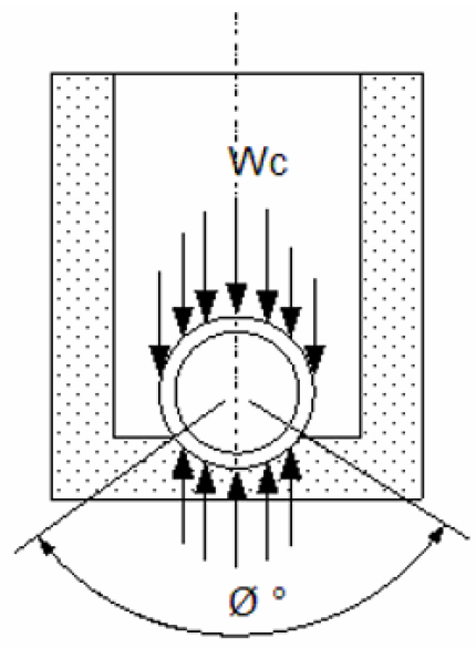
- Ө = Bedding angle of pipe (degrees)
- λ = Pipe moment of inertia (in4)
This is the uniformly distributed pressure on the pipe due to an equivalent point load at the surface that spreads at the soil distribution angle of 29.9 degrees from the surface point.
The longitudinal bending stress is given as:
(11)
\sigma_{L_bend}=\frac{M\cdot D}{2I}
\sigma_{L\_bend}=\frac{M\cdot D}{2I}Where:
- σL_bend = Longitudinal bending stress (psi)
The total longitudinal stress due to temperature differential is given as:
(12)
\sigma_{L_thermal}=E\cdot \alpha\cdot \Delta T
\sigma_{L\_thermal}=E\cdot \alpha\cdot \Delta TWhere:
- σL_thermal = Longitudinal thermal stress (psi)
- α = Coefficient of thermal expansion for steel (6.67×10⁻⁶ in/in deg F)
- △T = Temperature differential (installation – operation)
The total longitudinal stress, , is the sum of the stresses from internal pressure, soil load, surface loads, axial deflection, and temperature differential. The total longitudinal stress is compared to the allowable limit.
The combined equivalent (Tresca – Equation 14; von Mises – Equation 15) stress is calculated as:
(13)
\sigma_{E} = \max(|\sigma_{H_{Total}}|, |\sigma_{L_{Total}}|, |\sigma_{H_{Total}} – \sigma_{L_{Total}}|)
\sigma_{E} = \max(|\sigma_{H\_{Total}}|, |\sigma_{L\_{Total}}|, |\sigma_{H\_{Total}} - \sigma_{L\_{Total}}|)
(14)
\sigma_{E} = \sqrt{\sigma_{H_{Total}}^2 – \sigma_{H_{Total}} \cdot \sigma_{L_{Total}} + \sigma_{L_{Total}}^2}
\sigma_{E} = \sqrt{\sigma_{H\_{Total}}^2 - \sigma_{H\_{Total}} \cdot \sigma_{L\_{Total}} + \sigma_{L\_{Total}}^2}
Where:
- σE = Combined equivalent stress (psi)
Case guide
Part 1: Create Case
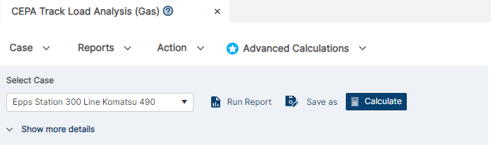
- Select the CEPA Track Load Analysis application from the Pipeline Crossing module
- To create a new case, click the “Add Case” button
- Enter Case Name, Location, Date and any necessary notes.
- Fill out all required Parameters.
- Make sure the values you are inputting are in the correct units.
- Click the CALCULATE button to overview results.
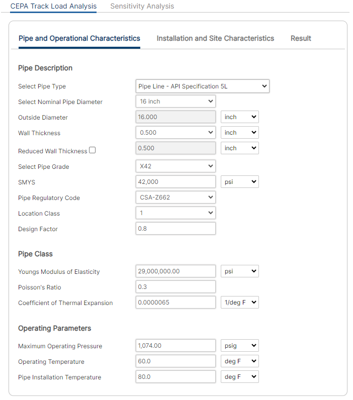
Input Parameters
- Nominal Pipe Size(in):(1/8” – 48”)
- Pipe Outside Diameter(in):(0.625” – 48”)
- Pipe Wall Thickness(in):(0.068”- >2”)
- Pipe Grade
- SMYS
- Pipe Regularly Code
- Location Class
- Design Factor
- Youngs Modulus of Elasticity
- Poisson’s Ratio
- Coefficient of Thermal Expansion
- Maximum Operating Pressure
- Operating Temperature
- Pipe Installation Temperature
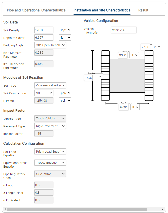
Installation and Site Characteristics:
- Solid Density
- Depth of Cover
- Bedding Angle
- Kb – Moment Parameter
- Kz – Deflection Parameter
- Soil Type
- Soil Compaction
- E Prime
- Vehicle Type
- Pavement Type
- Impact Factor
- Soil Load Equation
- Equivalent Stress Equation
- Pipe Regulatory Code
- Stress – Hoop
- Stress – Longitudinal
- Stress – Equivalent
- Vehicle Information
- Track Length
- Contact Width
- Vehicle Load
- Track Separation
Part 2: Outputs/Reports
- If you need to modify an input parameter, click the CALCULATE button after the change.
- To SAVE, fill out all required case details then click the SAVE button.
- To rename an existing file, click the SAVE As button. Provide all case info then click SAVE.
- To generate a REPORT, click the REPORT button.
- The user may export the Case/Report by clicking the Export to Excel icon.
- To delete a case, click the DELETE icon near the top of the widget.
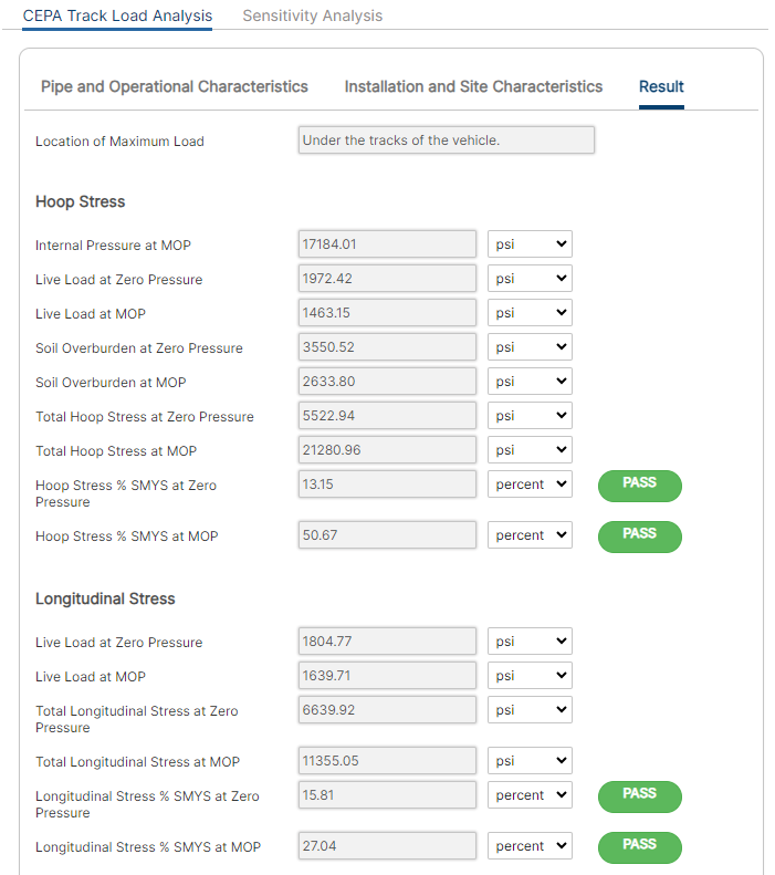
Results
Hoop Stress:
- Internal Pressure at MOP
- Live Load at Zero Pressure
- Live Load at MOP
- Total Hoop Stress at Zero Pressure
- Total Hoop Stress at MOP
- Hoop Stress % SMYS at Zero Pressure
- Hoop Stress % SMYS at MOP
Longitudinal Stress:
- Live Load at Zero Pressure
- Live Load at MOP
- Total Longitudinal Stress at Zero Pressure
- Total Longitudinal at MOP
- Longitudinal Stress % SMYS at Zero Pressure
- Longitudinal Stress % at MOP
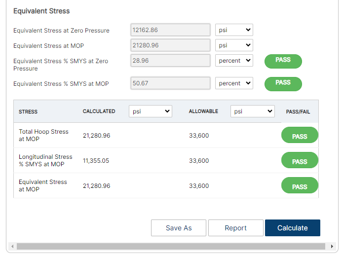
Equivalent Stress:
- Equivalent Stress at Zero Pressure
- Equivalent Stress at MOP
- Equivalent Stress % SMYS at Zero Pressure
- Equivalent Stress % SMYS at MOP
Results Table:
- Total Hoop Stress @ MOP
- Longitudinal Stress % SMYS @ MOP
- Equivalent Stress @ MOP
Reference
- “Canadian Energy Pipeline Association (CEPA) “Development of a Pipeline Surface Loading Screening Process and Assessment of Surface Load Dispersing Methods”, October 2009
FAQ
-
What are crossings – Live Load?
Many questions are asked about API 1102 regarding wheel load cyclic stresses on highways and railroads.
Live highway load, w, the load due to the wheel load at the highway surface. The load from only one wheel set needs to be considered. An axle is considered to have two-wheel sets.
Live rail load, w, pounds per sq inch, is the load applied at the surface of the crossing. It is assumed that the load is evenly distributed over an area that is 8’x 20’.The recommended default is 80,000 pounds (80 Kips) per axle. Check Out
-
Validation checks in place for API 1102 – Pipeline Crossing Railroad?
Below are the list of validation checks we have incorporated in API 1102 – Pipeline Crossing Railroad (Gas and Liquid). Check Out
-
Validation checks in place for API 1102 – Pipeline Crossing Highway?
Below are the list of validation checks we have incorporated in API 1102 – Pipeline Crossing Highway (Gas and Liquid). Check Out
-
Track Load – Interpolation Method (for Influence Coefficient)?
We recently issued an enhancement for Track load calculation by providing an option to use the Interpolation Method to calculate the Influence Coefficient (Ic). The old method calculated the Influence Coefficient using a roundoff method for ‘m-Influence Factor’ and ‘n-Influence Factor’ to get the Influence Coefficient from the table. Check Out
-
API 1102 Uncased Crossing 10 Foot Limit Understanding?
Uncased carrier pipe is subjected to internal loading from pressure and external loading from earth loading (dead load) and live (cyclic) loading from highway or railroad traffic. Other loading due to special or temporary conditions should be evaluated on the specific situation in the field (See Knowledge Base Article for Temporary Conditions). Check Out
-
Surface Load Mitigation Measures – Best Practice?
Method
Reduce the operating pressure of the pipeline.
Advantages
Provides a direct reduction of the hoop stress due to internal pressure. This reduction allows for additional circumferential stress due to equipment loads.
Disadvantages
– Reduces the beneficial effect of internal pressure on the pipe circumferential bending stresses due to fill and traffic loads.
– Could reduce the overall capacity of the pipeline and therefore should not be considered as a long term fix.
-
Difference between “Operating Weight” in Track Load Analysis and “concentrated surface load” in Wheel Load?
The term “Operating Weight” used in the track load analysis is a straight forward analysis as it takes the total weight of the equipment into consideration. We multiply the total weight by 0.5 to reflect the load on each track (see below the equation).
“Concentrated surface load” in the Wheel load calculation requires a more detailed understanding of the vehicle that is crossing. Below schematic will help better understand the requirement for “Concentrated surface load” entry in Wheel Load analysis.
-
Determining Trench Width for Crossings?
The basic analysis developed by M.G. Spangler includes frictional forces between the trench wall and the backfill. This permits the weight of the overburden to be partially carried by the surrounding soil and reduces the total soil load on the pipe. The equations require the following information to determine internal friction. Check Out
-
Combined Stress for Wheel Load and Track Load?
The question comes up from time to time how to address local stresses for wheel and track load calculations. ASME B31.8 833.9 Local Stresses states that the maximum allowable sum of circumferential stress due to internal pressure (Barlow Design Formula) and circumferential through-wall bending stress caused by surface vehicle loads or other local loads is 0.9ST, where S is the specified minimum yield strength, psi (MPA) per para. 841.1 (a), and T is the temperature derating factor per para. 841.1.8. Check Out
-
What Are Timber Mats in Crossing?
Timber mats are used for temporary access roads, work pads, staging areas, and to stabilize the ground beneath heavy equipment, dissipating heavy loads and providing equipment stability.
For short-term water crossings over narrow spans timber mats (also referred to as bridge mats) or crane mats may be an option.
For projects that require moving heavy equipment safely across pipelines, timber mats can be used to create air bridges which will support the weight of heavy equipment while protecting the pipelines below. Air bridges can also be used to cross culverts, ditches, or sensitive ground that needs to be bridged. Check Out
-
Redistributing Wheel and Track Loads (Pavement and Other Materials)?
This knowledge base article is a takeoff from “Pipeline Toolbox (PLTB) and Vehicles over Buried Pipelines – Maximum Allowable Stress”. These predictions through Spangler’s work, Battelle and others who contributed to validation makes PLTB one of most used programs in the industry. It includes temporary wheel and track load crossings that considers a uniformly distributed load at the surface while calculating the load on the pipe. This article will focus on concrete, asphalt and timber mats as well as other materials such as steel plates and composites. The other materials are not part of the Pipeline Toolbox which will be discussed. Check Out
-
Pipeline Crossings – External Loads and Vehicles over Buried Pipelines “Maximum Allowable Combined Stress”?
This article was created due to the number of inquiries regarding the Maximum Allowable Combined Stress for Class 3 Design Areas. The research by M. G. Spangler, Battelle and industry allowed this information to be a standard practice today with Wheel and Track Load analysis today. Check Out
-
Applicability of Class Location for Liquid Lines? What is the design factor used for Liquid Pipeline Operation?
Design factor specification for Liquid Pipelines are governed by ASME B31.4 Table 402.3.1(a)
Excerpts from B31.4: Check Out
-
Loading Requirements for API 1102 E-80 and E-90 Railroad Crossings?
API 1102 for railroad crossing program is based on the design methodology that has been used in analyzing existing uncased pipelines and designing new uncased pipelines that cross beneath railroads. This API design methodology relates to the train engine (E-80) which is the heaviest load: Check Out
-
What are Cased Crossings?
The pipeline industry begins to experience casing problems such as carrier pipe leaks/failures under road crossings.
- Atmospheric corrosion due to condensation (particularly at elevated temperatures and cold soils)
- Metal to metal shorts
- Electrolytic coupling or contact
Can the casing pipe protect the carrier pipe from external loadings? Check Out
-
Understanding Impact Factors in Pipeline Design (CEPA)
What is an Impact Factor?
An impact factor is a multiplier used in pipeline design to account for the additional stress caused by moving vehicles above the pipeline, compared to static loads. Think of it as a “safety buffer” that accounts for the dynamic nature of traffic. Check Out