Application Overview

This section provides a quick overview of the user interface which shows all basic components of software and explain the general procedure of performing analysis.

Launching the Software

The PRCI application is opened through the Technical Toolboxes menu. It would be displayed under On-Bottom Stability as it appears shown in Figure 2-1.

Creating New case

To create a new case for analysis, select the Case drop down menu. Then press the Create New Case button to open a prompt to save the new analysis(Figure 2-2).

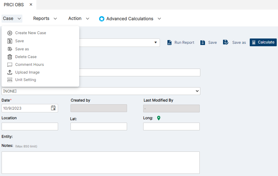
Browse to the desired directory and press the Save button to store the database in the selected location. Now that the database has been created in the required location, the main page radio button option will switch to Open. Select the analysis level and press the Start Program button.

Opening Existing Cases

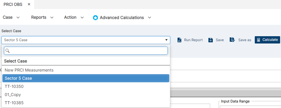
Open the Select Case drop down menu on the PRCI OBS application, all data will be immediately displayed in the parameters of the analysis.

Importing JSON File

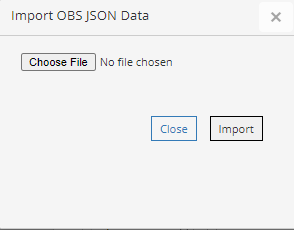
To import JSON Data Files, click the import button next to the green check mark in the calculation section. Then a a separate window will display with a Chose File and Import Option (Figure 2-3.5).

Main Window

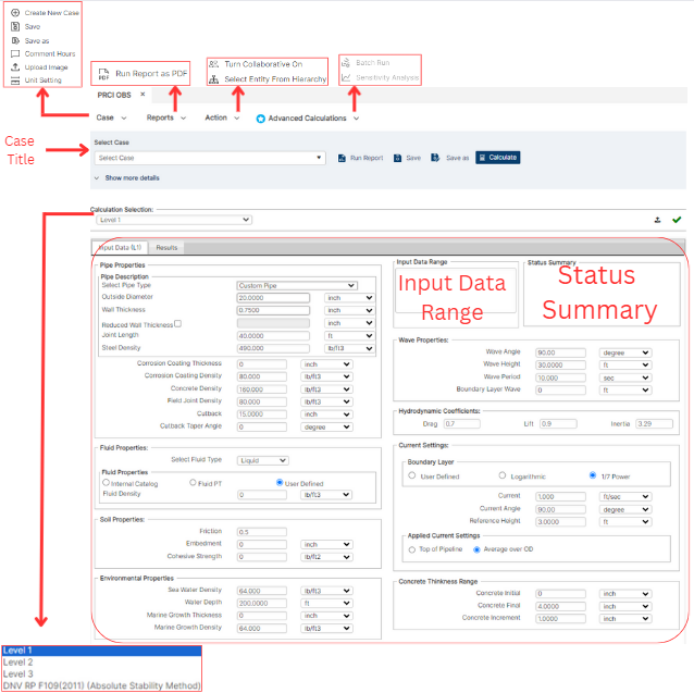
After launching the software and selecting the analysis, main window of the chosen analysis would appear. Main window is designed to cover all tools for managing cases, defining parameters, running, and generating reports and plots for different levels. All the operations are described throughout the manual, however, the more common items are presented here. These include navigation panel, toolbar, case navigation panel, input data tab, case definition, unit conversion, input data range, and status summary.

The Figure 2-4 illustrates an example of main window of PRCI software for a Level 1 analysis. This layout is more or less repeated other levels of the software, albeit with different input options as detailed in the relevant sections provided for each analysis level.

Calculation Selection

The Calculation Selection tab (Figure 2-5) provides a quick access to all levels of analysis as well as the software Main Menu. By clicking the Main Menu button, the software returns to Main Menu where users can load other projects or select other levels of analyses. Upon clicking other buttons in this tab, the software would switch directly to the corresponding analysis level.

Toolbar Description

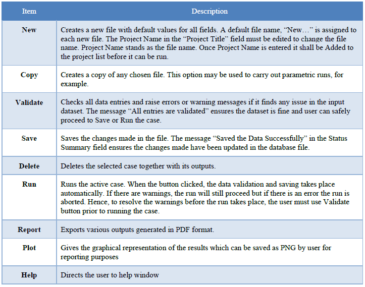
The Toolbar (Figure 2-6) includes standard commands for case-based operations such as creating, copying, deleting, saving, validating, running, and generating reports and plots.

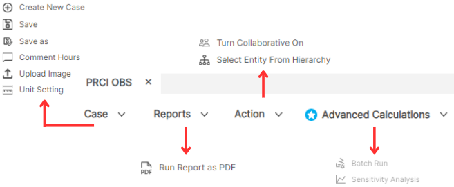
Table 2-1 presents descriptions of the various tools available in the software ribbon and common area.

Case Navigation Panel

All available Cases are displayed in Case Navigation Panel (Figure 2-4). The user can select a Case from this field to work on. Associated parameters’ values are displayed in Input fields once a selection is made.

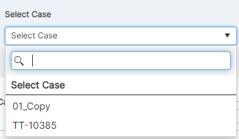
The Case List shows three main fields (Figure 2-7):

• Id: is a unique identifying number that database assigns to each individual case. The generated Input/output files are saved in a subdirectory identifiable by Id number as follows:
  \Results-Filename\Level1\Id
  The Filename is the name of created database (e.g. Example in the present case). Hence, the output files of Example Case (Id = 14) is located in:
  \Results-Example\Level1\14
• Case Name: is the name of created cases.
• Status: defines if the analysis for the case has been performed. It has two different states:
  ‘——’: No analysis is performed yet.
  ‘Done’: Analysis is completed.

The Case List is sortable as well. Users can sort the cases based on any of the three fields both in ascending and descending orders by clicking on the headers.

Input Data Tab

Input data tab, as shown in Figure 2-4, provides the entry data areas to define, modify, and display all input parameters of the selected case.

Case Title

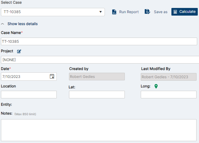
• Case Name: This field can be used to enter/modify the Case Name. Up to 50 alphanumeric characters (including special characters) can be entered in this field.

• Case Description: A short description of the case can be entered, such as pipeline details and other crucial data. Up to 50 alphanumeric characters (including special characters) can be entered in this field (Figure 2-8).

Unit Setting

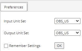
The software allows specification of the following unit systems for display of the input and output fields (Figure 2-9):

• Input
  • OBS_Metric (kilograms, meters and millimeters)
  • OBS_US (pounds, feet and inches)
• Output
  • OBS_Metric (kilograms, meters and millimeters)
  • OBS_US (pounds, feet and inches)

Upon changing the selection of the unit system, all inputs are converted automatically.

Input Data Range

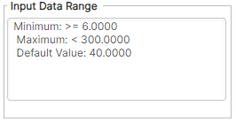
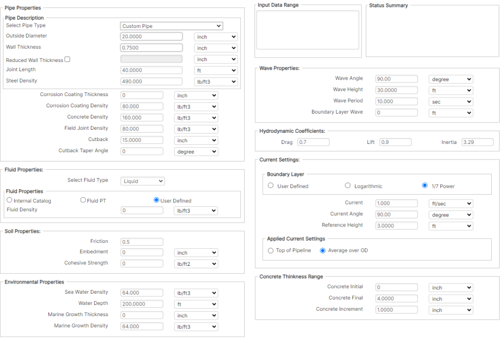
When an input field is selected, the area displays range and bound information for the minimum, maximum and default values of the current parameter selection. Figure 2-10 shows input data range for the Cohesive Strength field selection.

Status Summary

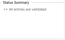
This field displays the status of any action carried out in the module such as error, successful analysis runs, and etc. (Figure 2-11).

Data Entry

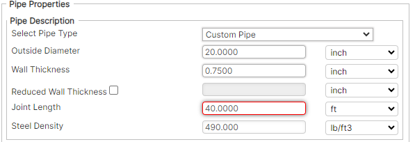
The input data can be specified, with the input fields selectable by mouse clicks, and able to be moved through by the standard TAB (forward) and SHIFT+TAB (backward) keyboard shortcuts. The Input Data Range field will display the minimum, maximum and default value for each numerical input, as well as the inclusiveness of the upper and lower bounds (Figure 2-10).

Procedure of Setting up a Case for Analysis

This section will briefly run through an example analysis, covering generic aspects such as the creation, setup, parameter definition, running, and report generation. The example is given for a Level 1 analysis to serve as a simple introduction to the PRCI software (as mention in 2.2).

Creating new Case

For a blank database file, the Case Navigation area is initially filled with two default cases (one in English unit and the other in SI unit). Users can directly run these default cases, or they can create a copy of these cases in order to create a new case.

Alternatively, to create a fresh new case within the database (and for later adding more cases within the same database), press the New button at the very left of the toolbar (Figure 2-6), which will open the Unit Settings dialog (Figure 2-12).

Select the desired system of units (this example has selected SI units). By clicking OK button, a new case would be created in the database with default entry values (Figure 2-13) and a default name of “New Case – (1)”. The Case Description field remains empty. These two fields can be changed and saved, as shown in Figure 2-8.

The new case would be added to the Case List Table.

Date Entry

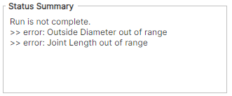
If a value is entered outside the allowable bounds (or in a different format than required, e.g. text when a number is requested) as indicated in the Input Data Range field, once the Validate button is clicked (Figure 2-6), a corresponding error message would appear in the Status Summary field (Figure 2-14). Validate button can be used regularly to perform a basic check on correctness of data entries. It is also recommended to use this button prior to saving and/or running the case. As shown in Figure 2-14, the error message in Status Summary, specifically declares which field(s) is problematic.

However, the validation check mostly performs a single entry check and does not always guarantee a smooth run for a set of input data. This is because, depending on selected analysis, a successful run depends on the interactions of many parameters and iterative solutions of some equations.

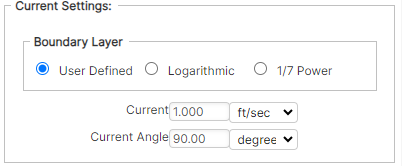
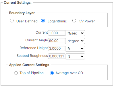
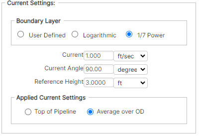
Some of the input data are optional where the user can choose via selecting a radio button. Depending on the selection, additional fields may appear in the input tab. For example, see choices in the Current Settings box of Input Tab as presented in Figure 2-15. The User Defined option displays only two required entries (Current and Current Angle). By selecting 1/7 Power, additional entry fields would appear, while selecting the Logarithmic Boundary Layer formulation, would add an extra field to specify Seabed Roughness.

Running the Analysis and Creating Reports

Now that all the input data is specified, and the project is validated and saved, press the Run button to run the analysis (Figure 2-6).

The software will compute the results, and the Output Data (L1) tab is displayed when the run has completed (Figure 2-16). Accordingly, the status of the case in Case List would turn to “Done” as shown in Figure 2-16.

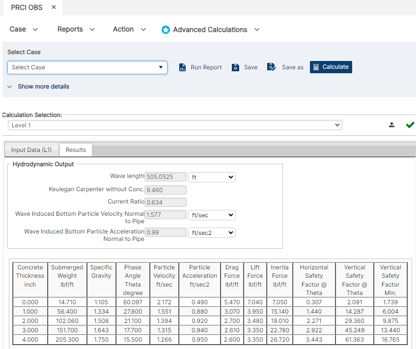
As the Run completes successfully, a PDF report file would also be generated automatically. The PDF file could be opened through the Report button (Figure 2-6).

Copying and Deleting Case

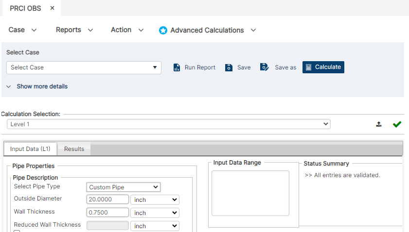
Upon completion of a run and returning to the Input Data tab (by clicking on the tab list or by using the standard CTRL+TAB and CTRL+SHIFT+TAB keyboard shortcuts) it is noticed that the Input Data entries has turned to Read-Only (Figure 2-17). This occurs in order to ensure that the input data cannot be changed accidently and remain in consistent with the output data. The only fields that can be altered and saved are the Case Name and Case Description. If users want to alter some entries of the case and see the outputs, they need to create a Copy of the case and alter the entries and re-Run the case. This approach might improve in the future upgrades of the software.

Creating a copy of selected case in the List Case field is accomplished by clicking the Copy button (Figure 2-6). This may be particularly useful for running sensitivity cases on single parameters, or for keeping a backup of a working project when attempting to determine other viable input options. The copied case will, by default, carry the parent case name with “-Copy1)” appended.

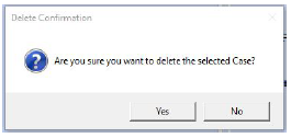
A Case may also be removed from the database by selecting them in the List Case field and pressing the Delete button, which prompts a confirmation message before case deletion (Figure 2-18).

Generating Plots

The generation of plots is performed in a similar manner to the generation of the output reports shown in Section 2.3.3. Once all the input values for the analysis are specified and the analysis has been run, the Plots button in the ribbon can be selected (Figure 2-6). The plotting features depend on the selected analysis and will be detailed in the relevant section of this manual.

References

1. Verley, R. L. P. and Lund, K. M. A Soil Resistance Model for Pipelines Placed on Clay Soils, OMAE – Volume 5, 1995
2. DNV-RP-F109, On-Bottom Stability Design of Submarine Pipelines, Det Norske Veritas, Nov-2011
3. Ochi, M. K. Hubble, E.N. Six-parameter wave spectra, Proceedings 15th International Conference on Coastal Engineering, Honolulu, 1976
4. DNV-OS-F101, Submarine Pipeline Systems, Det Norske Veritas, Oct-2013
5. On-Bottom Stability in Deep Waters Note, Det Norske Veritas
6. Catalog No. L51522e, PR-170-185, Hydrodynamic Forces on Pipelines: Model Tests, Prepared for PRCI by the Danish Hydraulic Institute, Dec-1986
7. PR-170-716, Hydrodynamic Forces Acting on a Pipeline in an Open Trench, Prepared for PRCI by the Danish Hydraulic Institute, Jan-1988
8. Ochi, M. K. and Hubble, E.N. Six-Parameter Wave Spectra, Proceedings 15th International Conference on Coastal Engineering, Honolulu, 1976
9. Mardia, K. V., Statistics of Directional Data. London: Academic Press, 1972
10. Borgman L.E., Directional Wave Spectra from Wave Sensors. In: Earle M.D., Malahoff A. (eds) Ocean Wave Climate. Marine Science, vol 8. Springer, Boston, MA, 1979
11. Mardia, K.V., Some properties of clasical multi-dimesional scaling,Communications in Statistics – Theory and Methods, 1978
12. PR-169-186
13. PR-175-420
14. Catalog No. L51570e, Contract PR-194-719, Energy Based Pipe-Soil Interaction Models, PRCI, June 1988
15. PR-162-157
16. PRCI Project PR-178-04405, Submarine Pipeline On-Bottom Stability Volume 1: Analysis and Design Guidelines, Kellogg Brown & Root, Inc., Dec-2008
17. PRCI Project PR-178-04405, Submarine Pipeline On-Bottom Stability Volume 2: Analysis and Design Guidelines, Kellogg Brown & Root, Inc., Dec-2008
18. Abdolmaleki, K. and Gregory, C. J., Performance of Pipe-Soil Interaction Models in a Quasi-Dynamic Approach to Pipeline Stability Analysis, OMAE-77988, 2018, Spain
19. Jacobsen, V., Bryndum, M.B., and Bonde, C., “Fluid Loads on Pipelines: Sheltered or Sliding,” Proc. 21st Offshore Technology Conference, Paper No. OTC 6056, Houston, 1989

FAQ

---