
Introduction
Used for primarily water lines associated with production facilities. Limited to Reynolds numbers in the range of Re = 4,000 to 1,000000. Its chief drawback is that the Hazen-Williams coefficient is largely an experience factor which also depends on the viscosity of the product flowing.
Formulas
Downstream Pressure
P_2=P_1-GL\bigg( \frac{B}{0.006171C_{HW}D^{2.63})^{1.852}} \bigg)-\triangle H
P_2=P_1-GL\bigg( \frac{B}{0.006171C_{HW}D^{2.63})^{1.852}} \bigg)-\triangle HFlow Rate
B=0.006171C_{HW}D^{2.63}\bigg[ \frac{P_1-P_2-\triangle H}{GL} \bigg]^{0.54}
B=0.006171C_{HW}D^{2.63}\bigg[ \frac{P_1-P_2-\triangle H}{GL} \bigg]^{0.54}Internal Diameter
D=\bigg( \frac{0.006171C_{HW}(P_1-P_2-\triangle H}{(GL)^{0.54}} \bigg)^{0.38} \~\\triangle H=0.433514G(H_2-H_1) \~\ \triangle P=\frac{(P_1-P_2- \triangle H)}{L}
D=\bigg( \frac{0.006171C_{HW}(P_1-P_2-\triangle H}{(GL)^{0.54}} \bigg)^{0.38} \\~\\\triangle H=0.433514G(H_2-H_1) \\~\\ \triangle P=\frac{(P_1-P_2- \triangle H)}{L}Upstream Pressure
P_1=P_2+GL\bigg( \frac{B}{0.006171C_{HW}D^{2.63})^{1.852}} \bigg)-\triangle H
P_1=P_2+GL\bigg( \frac{B}{0.006171C_{HW}D^{2.63})^{1.852}} \bigg)-\triangle H𝐶𝐻𝑊 – Hazen − Williams Coefficient
𝐻1 − Upstream Elevation[ft]
𝐻2 − Downstream Elevation[ft]
𝐻 − Head Loss[ft]
𝐷−Pipe Internal Diameter[in]
𝐿 − Pipeline Length[mi]
𝐺 − Liquid Specific Gravity
∆𝑃 − Pressure Drop[psi/mile]
𝑃1 − Upstream Pressure[psig]
𝑃2 − Downstream Pressure[psig]
Case Guide
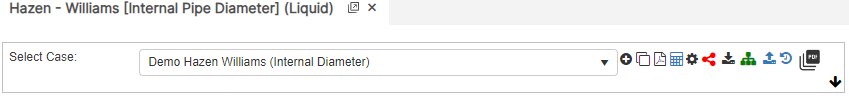
Part 1: Create Case
- Select the Hazen – Williams application in the Hydraulics module.
- To create a new case, click the “Add Case” button.
- Enter Case Name, Location, Date and any necessary notes.
- Fill out all required parameters.
- Make sure the values you are inputting are in the correct units.
- Click the CALCULATE button to overview results
Input Parameters
- Temperature base(°F)
- Pressure base(psia)
- Gas Flowing Temperature(°F)
- Gas Specific Gravity
- Compressibility Factor
- Pipeline Efficiency Factor
- Upstream Pressure(psig)
- Downstream Pressure(psig)
- Flow Rate(Barrels per Day)
- Internal Pipe Diameter(in)
- Length of Pipeline(mi)
- Upstream Elevation(ft)
- Downstream Elevation(ft)
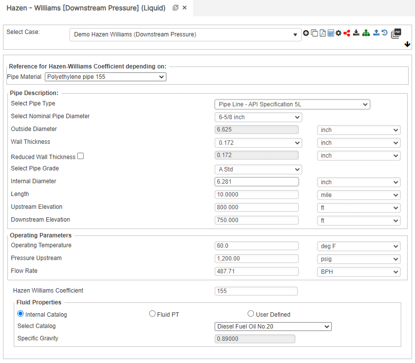
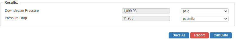
Downstream Pressure
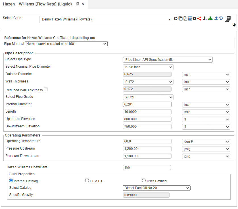
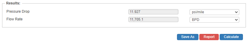
Flow Rate
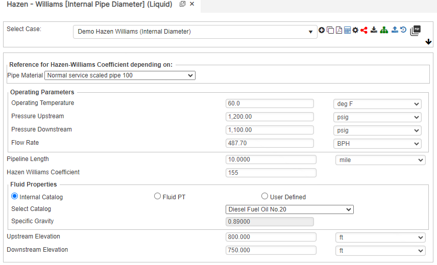
Internal Pipe Diameter
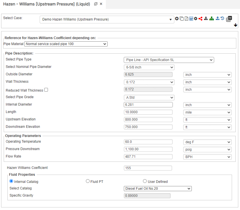
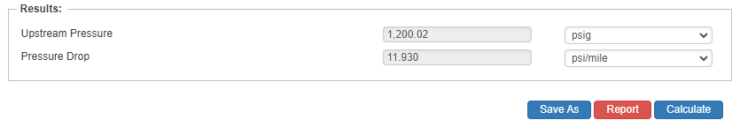
Upstream Pressure
Part 2: Outputs/Reports
- If you need to modify an input parameter, click the CALCULATE button after the change.
- To SAVE, fill out all required case details then click the SAVE button.
- To rename an existing file, click the SAVE As button. Provide all case info then click SAVE.
- To generate a REPORT, click the REPORT button.
- The user may export the Case/Report by clicking the Export to Excel icon.
- To delete a case, click the DELETE icon near the top of the widget.
Results
- Pressure Drop(psi/mile)
- Downstream Pressure(psig)
- Flow Rate(Barrels per Day)
- Internal Pipe Diameter(in)
- Upstream Pressure(psig)
Downstream Pressure

Flow Rate

Internal Pipe Diameter

Upstream Pressure

References
- “Pipeline Rules of Thumb” Gulf Professional Publishing, Seventh Edition, McAllister, E. W.
- “Gas Pipeline Hydraulics”, Systek Technologies, Inc., Menon, Shahi E.
- “Advanced Pipeline Design”, Carroll, Landon and Hudkins, Weston R.
- American Gas Association (AGA), “Reference: Eq-17-18, Section 17, GPSA”, Engineering Data Book, Eleventh Edition
- Hydraulic Transients, McGraw-Hill, New York., Streeter, V.L. and Wylie, E.B. (1967)
- Water Hammer Analysis. Jour. Hyd. Div., ASCE., Vol. 88, HY3, pp79-113 May, Streeter, V.L. (1969)
- Unsteady flow calculations by numerical methods’, Jour. Basic Eng., ASME., 94, pp457-466, June. Streeter, V.L. (1972),
- Hydraulic Pipelines, John Wiley & Sons, J. P Tullis (1989)
FAQ
-
What is Erosional Velocity?
Pipe erosion begins when velocity exceeds the value of C/SQRT(ρ) in ft/s, where ρ = gas density (in lb./ft3) and C = empirical constant (in lb./s/ft2) (starting erosional velocity). We used C=100 as API RP 14E (1984). However, this value can be changed based on the internal conditions of the pipeline. Check Out
-
What is Sonic Velocity?
The maximum possible velocity of a compressible fluid in a pipe is called sonic velocity. Oilfield liquids are semi-compressible, due to dissolved gases. Check Out