Level 3 Analysis

Introduction

In a Level 3 analysis, a two-dimensional dynamic pipeline model is used to calculate stresses and deflections in the line during storm conditions. Input parameters are specified over a grid, taking account of lengthwise variations along the pipeline route. A time history of the on-bottom current velocities and wave kinematics is simulated by the software module to model the pipeline behavior in irregular seas. The pipeline model considers the effect of end restraints such as risers and anchor points by modeling them as a series of springs on the end of the pipeline.

It is anticipated that this type of analysis will be used to establish a refined design, or to check and/or calibrate designs produced using a Level 2 analysis, particularly where the Level 2 assumptions do not accurately represent the actual situation. This may occur close to end restraints or other structural restraints, if axial tension could develop, or if excessive pipe movements are allowed.

The Level 3 software module consists of multiple tabs for specification of inputs, controls for the viewing and plotting of results, and three core calculation submodules: WINWAVE, the Random Wave Generation module; WINFORCE, the Hydrodynamic Force module; and WINDYNA, the dynamic simulation module.

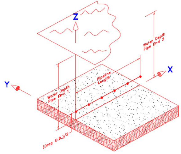
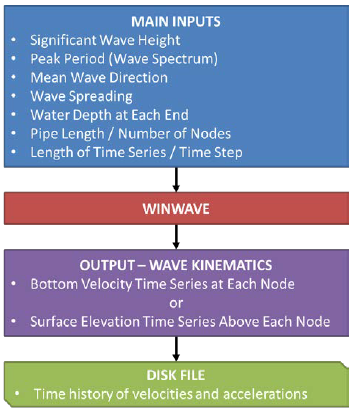
The Random Wave Generation module WINWAVE simulates water-particle velocity time series that result from wave motion at the sea surface. The time series are simulated at grid points on the sea floor that correspond to the pipeline route. The geometric layout of the pipeline and nodes is shown in Figure 5-1. The velocity time series simulated at each pipe node is passed to the hydrodynamic force module. Plot output of the velocities is available and can be referenced to check the simulation output.

The main assumption of the Level 3 analysis tool is that the Fourier expansion of the measured drag and lift forces in regular waves (as determined during the PRCI model tests, project PR-170-185 [6]) can be used to calculate the forces associated with the individual waves in irregular waves when taking into account the effect of the flow history; the so-called “wake effect”.

Calculation Procedure

The Level 3 suite consists of a top level input and post processing module and an integrated time domain dynamic simulation routine that incorporates random wave generation and hydrodynamic forces based on Fourier decomposition of results from numerous model tests and soil models which include lateral earth pressure soil resistance as well as frictional soil resistance. Three core subroutines of the Level 3 module are WINWAVE, WINFORCE and WINDYNA.

The random wave generation routine (WINWAVE) calculates bottom water particle velocities based on Airy wave theory and a set of randomly phased waves that are assigned different wave frequencies and directions. Wave energy is directionally spread using a wrapped normal distribution. Each component wave is assigned a direction based on a normal distribution in which the mean direction and standard deviation from the mean direction are specified by the user.

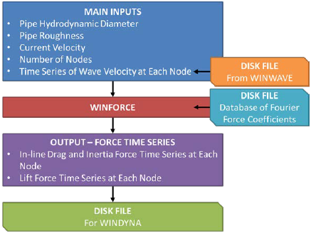
The hydrodynamic force generation routine (WINFORCE) uses the generated bottom particle velocities and a state-of-the-art force formulation to calculate hydrodynamic drag and lift forces on a stationary pipeline. The calculation uses a Fourier summation to determine the wave forces. The coefficients for the Fourier summation are taken from a database developed from the model test results. The three database files of force coefficients (AGAWCU, AGAWCX, and AGAWU) that were developed for PRCI are incorporated in the Level 3 module.

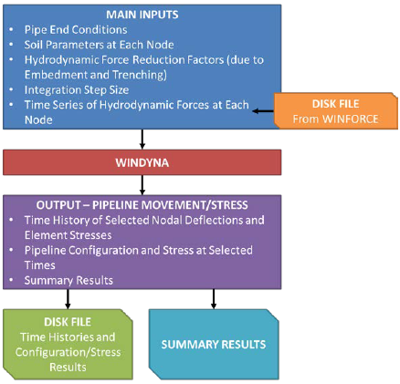
The on-bottom pipeline dynamics simulation routine (WINDYNA) models the pipeline as two-dimensional finite beam elements. The module uses the hydrodynamic forces and a history dependent soil resistance model (developed for the PRCI in project PR-194-719 [14]) to dynamically model the wave/soil interaction. All elements are in a straight line and of equal length, but soil parameters, pipe parameters, boundary conditions, and applied loads can be varied along the pipe length.

Pipeline displacements, embedment, instantaneous factors of safety and stresses are the main outputs. These can be obtained for several nodes as a function of time, or for the entire pipeline at specified time steps.

The processes within the Level 3 module are illustrated in Figure 5-2, Figure 5-3, and Figure 5-4.

Guidance Notes

General

Whereas the Level 2 and ASM modules may be used for routine determination of pipeline stability and selection of concrete thickness, Level 3 is not as well suited to those tasks. Instead, it does offer the potential for optimizing pipeline stability with respect to concrete weight coating, using a more refined but complex analysis than that used by the other levels. Before embarking on a stability analysis using the Level 3 module, the detailed internal procedures should be well understood, including some of the following points:

• Preliminary stability analyses should be completed using Level 2 or the ASM module, so as to have a good starting point for a Level 3 stability analysis.
• For each pipe outer diameter and weight, sufficient runs need to be made with different “seeds”. Random seeds are numbers used as internal input to generate random irregular sea states, with two different seed values resulting in two different sea states. Performing the analysis with a sufficient number of storm simulation seeds provides a reliable indication of the range of results which may be obtained for the specified wave spectrum parameters.

Note: This may need to be repeated at other water depths and wave conditions along the pipeline route.

• Once a satisfactory pipe weight and outer diameter have been determined for one condition, say the maximum significant wave height (Hs) case, other wave conditions need to be checked e.g. storms with lower Hs but greater peak period and/or different peakedness. Add some additional cases to check the effects of currents. These all need to be run with sufficient different seeds.

Note: This may need to be repeated at other water depths and wave conditions along the pipeline route.

• Instead, the criteria for pipeline stability need to be established. With Level 3 the instantaneous factors of safety computed are not meaningful. The following questions need to be answered:
  • What displacement is acceptable?
  • If a single 3-hour storm produces displacements greater than a minor fraction of the pipeline diameter, what will be the total displacement (and resulting stresses) of the pipeline during a lifetime of storms and how can that be determined?
• Level 3 reflects many kinds of nonlinear behavior as discussed further below. It is not rare for this to produce unexpected results which then require further evaluation and time.
• Due to Level 3’s greater complexity, there is a larger potential for errors in the usage of Level 3 as compared to the other levels, as well as greater difficulty in identifying the errors.

In summary, the stability analysis using Level 3 will require additional time and effort compared to that using Levels 1, 2 or ASM. Additionally, Level 3 assessment is more suitable for experienced users who are able to provide at least engineering judgement on the results. However, this may be beneficial depending on the case considered, with the decision of design approach left up to the designer.

Simulations with Unit Length

One way to minimize the complexity of a Level 3 analysis whilst still claiming the benefits of the more advanced stability analysis is to simulate a single pipe segment of unit length. This allows one to determine if a unit length of pipe would remain in place using all of the hydrodynamics, force estimation, and soil embedment resistance of the dynamic simulation without the additional output and runtime burden of multiple segments. Importantly, simulations with unit length can provide a very good source of information on the physical behavior of the considering design case.

Non-Linearities

The Level 3 module has a great number of the non-linearities that reflect corresponding physical non-linearities. The software module evaluates pipeline stability every few degrees during wave cycles. Unexpected results almost always are associated with shifts in the relationship between drag and lift forces, i.e. the phase in the wave cycle at which the critical conditions occur changes due the non-linearities. Consequently, small changes in parameters can shift the relationship between drag and lift forces in such a way that the general trends one expects do not apply. This is especially true for relatively shallow water cases, say less than 200 ft. It is always good to study variations around the design parameters. Unfortunately, the design parameter space for pipeline stability is large enough that to do this systematically is considerable work that is difficult to justify (and may produce results that are even more difficult to explain!).

Simulation Duration

In order for the results of a particular Level 3 simulation to be representative, it is necessary to simulate a sufficient length of time. Typically, this means that Level 3 simulations should be made to represent on the order of three hours of time. If shorter periods of time are simulated, the likelihood that the extreme waves are included in the analysis is reduced. Moreover, since the pipe/soil interaction is history dependent, a single 3-hour simulation may not be representative of the “average” result determined from a large number of simulations, where each simulation represents a different realization of the design sea state. This is most likely to be the case in weaker soils, where the history dependent portion of the soil resistance can become very large in relation to the history independent portion. If the pipe breaks out of the soil during such a simulation, a large change in total soil resistance capability would occur, since the history dependent portion is reset to zero. For this type problem, the timing of the breakout (early or late in the simulation) could significantly change the total net movement of the pipe.

Further Comments on Displacement

The resulting pipe displacements obtained from a Level 3 analysis should be used with caution. The pipeline-soil interaction tests that the calculation routines are based on (see Chapter 1 of [16]) were conducted by oscillating a short length of pipe back and forth on a prepared bed so that it would become embedded, and then determining the force required to pull it out of the trench it had created. The focus of these test programs was not to determine how far the pipe would move. The amount of movement calculated by the software is a function of how many times the wave force exceeds the force to move the pipe from the embedment trench that develops after each movement. The Level 3 analysis has not been validated as to the amount of pipeline displacement produced by specified wave and soil conditions, i.e. as to the accuracy of the displacement prediction. These test programs and the resulting calculation routines such as those used by the Level 3 module were developed to determine the weight of pipeline needed to remain stable as-laid. Any estimate they produce as to the amount of displacement to be experienced needs to be treated with caution.

Case Definition Tab

This Input Data tab defines the case title, simulation duration, unit system, pipe properties and water depths, as presented in Figure 5-5.

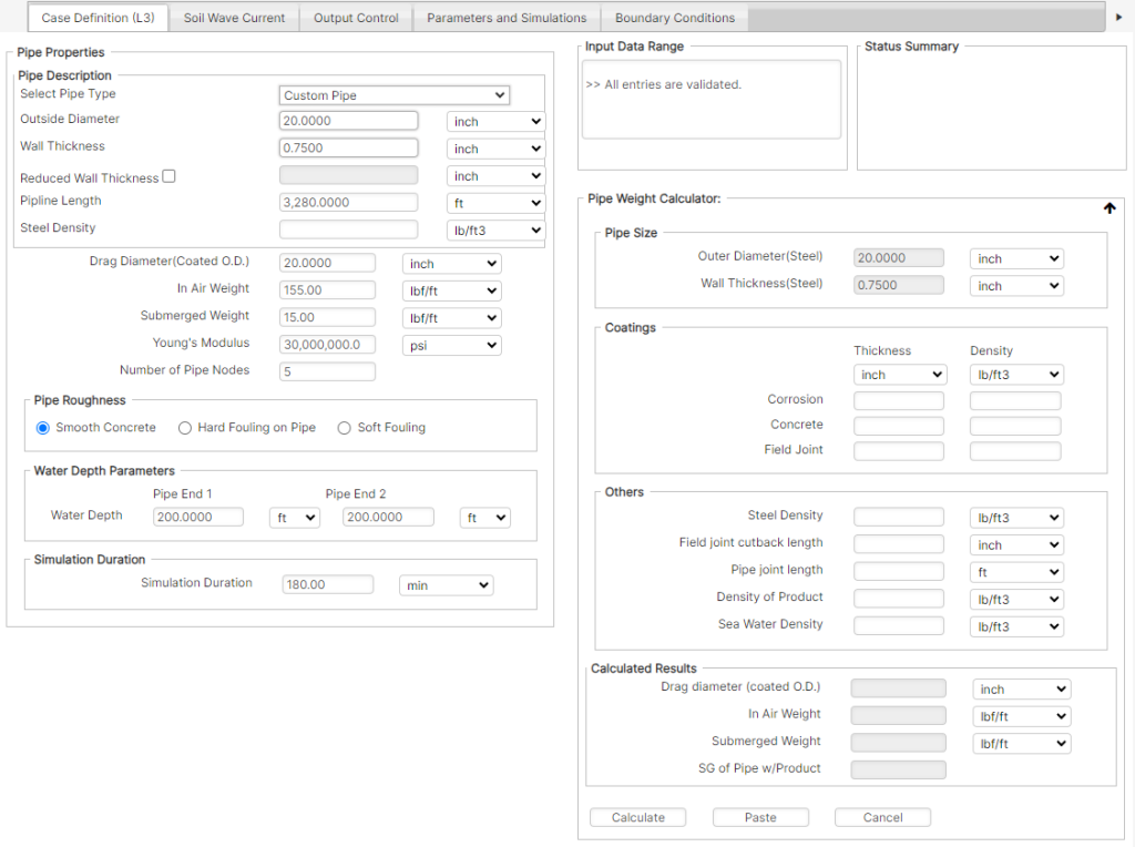
Pipe Properties

Outer Diameter -The outer diameter of the steel pipe.
Wall Thickness – The wall thickness of the steel pipe.
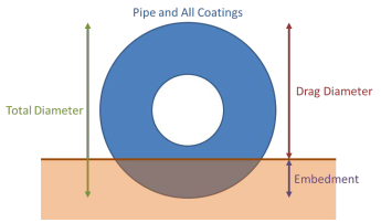
Drag Diameter (Coated OD) – Total pipe hydrodynamic diameter, including all coatings, that is not embedded in the soil (refer to Figure 5-6). This may also be input using the Pipe Weight Calculator option.

In-Air Weight – Average total weight of the pipeline, including all coatings and contents, in air per unit length of pipe. This may also be input using the Pipe Weight Calculator option.
Submerged Weight – Average total submerged weight of the pipeline, including all coatings and contents, per unit length of pipeline. This value is equal to the in-air weight minus the buoyant force of displaced water. This may also be input using the Pipe Weight Calculator option.
Young’s Modulus – Young’s Modulus for the steel pipe.
Pipe Roughness – External roughness ratio of the outermost surface of the pipe, selectable from the following [6]:

• Concrete: smooth concrete coating; k/D = 10^-3
• Roughened: A roughened concrete coating (typically resulting from hard bio-fouling, such as barnacles); k/D = 10^-2
• Very Rough: further roughened pipe (typically resulting from soft bio-fouling); k/D = 5·10^-2

Pipeline Length – The total length of pipeline to be analyzed. If only a section of pipe is to be analyzed for stability (similar to a Level 2 analysis), a unit length of pipeline (a one foot or one meter segment of pipe) is sufficient.
Number of Pipe Nodes – The number of nodal points to include in the finite element model. If only a section of pipe is to be analyzed for stability (similar to a Level 2 analysis), a two-node model (which corresponds to a single element model) is sufficient.
Water Depth Parameters – The water depth at the first end and the second end of the pipeline.
Simulation Duration – The simulated duration (not to be confused with the computing runtime) is the total duration for the dynamic simulation of the design storm. Based on limitations of the Random Wave Generation module, durations must be no greater than 1000 cycles (based on the peak period). In order for the results of a particular simulation to be representative, it is necessary to simulate a sufficient length of time.

Pipe Weight Calculator

This dialog box enables calculation of pipe weight parameters such as the in-air weight, the submerged weight and the specific gravity of the pipe with product contents, with the following operation buttons, as presented in Figure 5-7:

• Calc Button
  • Performs the calculation of the following parameters based on the input values.
• Paste Button
  • Results from the Pipe Weight Calculator may be pasted into the Pipe Properties section of the input by using the Paste button.
• Cancel Button
  • The calculation may be canceled without pasting the information into the Pipeline Parameters section of the input by selecting the Cancel button.

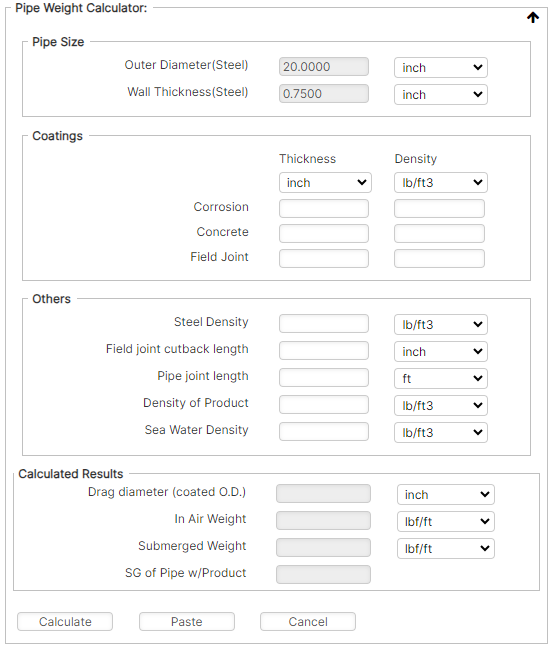
Pipe Size

Outer Diameter -The outer diameter of the steel pipe.
Wall Thickness – The wall thickness of the steel pipe.

Coatings

Corrosion Coating Thickness – Thickness of the external corrosion (or insulation) coating.
Corrosion Coating Density – Density of the external corrosion (or insulation) coating.
Concrete Coating Thickness – The thickness of the external layer of concrete coating to be considered.
Concrete Coating Density – Density of the external concrete weight coating.
Field Joint Coating Thickness – The thickness of the field joint coating to be considered.
Field Joint Coating Density – Density of the field joint coating and infill.

Others

Steel Density – Density of the steel pipe.
Field Joint Cutback Length – The Pipe Weight Calculator assumes a taper angle of 0° from the radial direction of the pipe.
Pipe Joint Length – The nominal length of one pipe joint.
Density of Product – Density of the product/contents inside the pipeline.
Seawater Density – Density of the seawater at the pipe location.

Calculated Result

Drag Diameter (Coated OD) – The total outer diameter of the pipe with all coatings.
In-Air Weight – The total of the pipe weight, concrete and corrosion coating weight without field joint coating weight and the internal contents (product weight), as an average per unit length. The ratio of field joints and concrete/corrosion coating is specified with the cutback length and pipe joint length.
Submerged Weight – The in-air weight minus the buoyancy force from the displaced seawater on the coated pipe (drag OD).
Specific Gravity of Pipe with Product – The specific gravity is presented for information purposes only, calculated as the ratio of the in-air weight of the pipe to the buoyancy force.

Soil Wave Current Tab

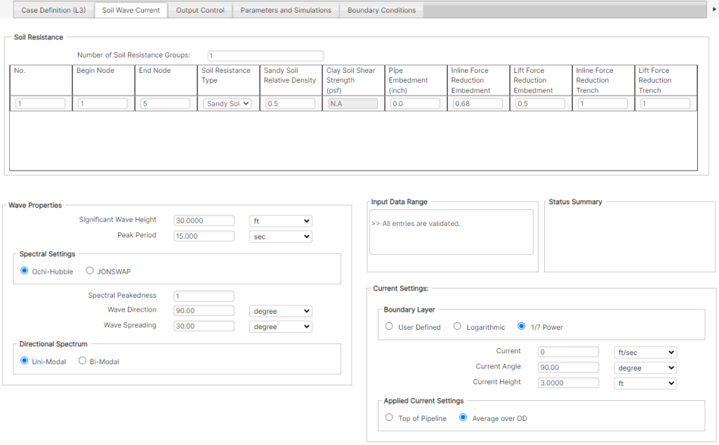
Soil Resistance

Number of Soil Resistance Groups – The soil conditions can be varied over the length of the pipeline. The user may input up to a maximum of ten different soil groups.
Begin Node – Beginning node number for the soil group.
End Node – Ending node number for the soil group.
Soil Resistance Type – The model for determination of lateral earth pressure soil resistance and frictional soil resistance using the PRCI pipe/soil interaction model is selectable from the options of sandy soil and clay soil. The user should note that the V&S and V&L models have not been implemented in the Level 3 and the existing soil models are still the original PRCI models. This is crucial when it is planned to compare the results of Level 2 and Level 3.
Sandy Soil Relative Density – This field will be inactive when clay soil is chosen.
Clay Soil Shear Strength – This field will be inactive when sandy soil is chosen.
Pipe Embedment – If this value is positive, it represents the limiting pipe embedment into the soil. If this value is negative (or zero), it represents the actual pipe embedment at the start of the run.
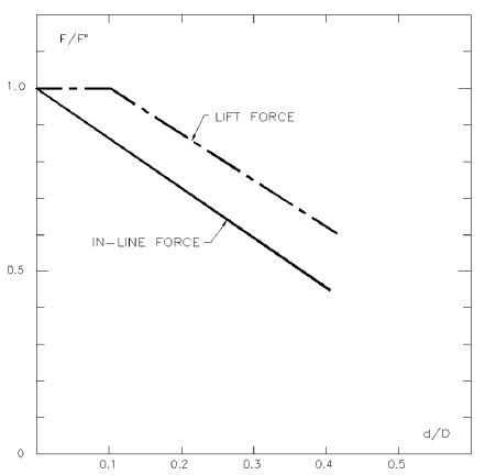
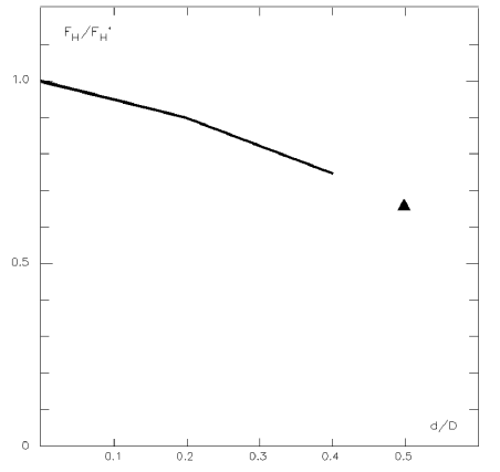
In-Line Force Reduction due to Embedment (Level 3) – Maximum in-line force reduction multiplier due to pipe embedment. Considering the reduction factor data presented in Figure 5-9 and Figure 5-10, the following values may be generally suggested for the available soils at an embedment ratio of 0.5:

• 0.313 for clay
• 0.680 for sand

Lift Force Reduction due to Embedment (Level 3) – Maximum lift force reduction multiplier due to pipe embedment. Considering the reduction factor data presented in Figure 5-9, the following values may be generally suggested for the available soils at an embedment ratio of 0.5, as per [6]:

• 0.5 for clay
• 0.5 for sand

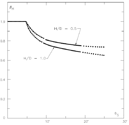
In-Line Force Reduction due to Trench (Level 3) – Maximum in-line force reduction multiplier due to trench geometry. This value may be obtained using the reduction factor data presented in Figure 5-11. The reduction factor is plotted against the trench slope measured with respect to the flat seabed. The dotted lines represent extrapolations to the actual conducted model tests.

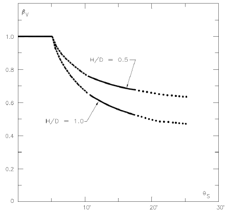
Lift Force Reduction due to Trench (Level 3) – Maximum lift force reduction multiplier due to trench geometry. This value may be obtained using the reduction factor data presented in Figure 5-12. The reduction factor is plotted against the trench slope measured with respect to the flat seabed. The dotted lines represent extrapolations to the actual conducted model tests.

Wave Properties Input Type

The wave type is specified from two options: Surface Wave Spectra and Near Seabed Velocity.

Surface Wave Spectra – The wave is defined by the surface wave parameters, which are used to calculate the wave loads near the seabed:

• Significant Wave Height: the vertical distance from trough to crest of the significant wave.
• Peak Period: the time interval between successive peak wave crests passing a particular point.

Near Seabed Velocity – The wave is defined by the near-seabed parameters:

• Significant Velocity: the velocity of the near seabed wave-induced current.
• Zero-Crossing Period: period of the near seabed wave-induced current.

Wave Properties Spectral Settings

The spectral settings are available for the wave input selection of Surface Wave Spectra.

Ochi-Hubble – This is a general spectrum formulated to describe seas as a combination of two different sea states, using a sum of two Gamma distributions [3]. The Ochi-Hubble spectrum is modelled in the software as a single peak spectrum, and is defined by the following parameters, as presented in Figure 4-11:

• Spectral Peakedness: the dimensionless peakedness parameter for the Ochi-Hubble spectrum.
• Wave Direction: the angle of wave propagation relative to the pipeline (perpendicular to the pipe is 90°).
• Wave Spreading: the standard deviation of wave spreading used in the wrapped normal spreading function.

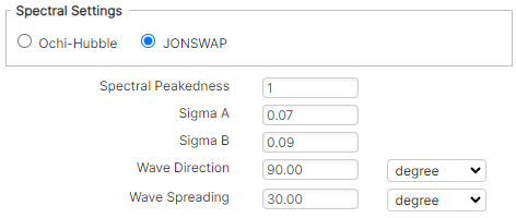
JONSWAP – This single peak spectrum was initially formulated as a modification of the Pierson-Moskowitz spectrum to describe a developing sea state in a fetch limited situation. It is often applied to on-bottom stability analyses, and is defined by the following parameters, as presented in Figure 4-12.

• Spectral Peakedness: The dimensionless peakedness parameter for the JONSWAP spectrum.
• Sigma A: JONSWAP spectral width parameter, applicable when 𝜔≤𝜔_𝑝.
  Where:
  • ω is the wave angular frequency
  • ω_p is the wave angular spectral peak frequency
• Sigma B: JONSWAP spectral width parameter, applicable when 𝜔>𝜔_𝑝.
• Wave Direction: the angle of wave propagation relative to the pipeline (perpendicular to the pipe is 90°).
• Wave Spreading: the standard deviation of wave spreading used in the wrapped normal spreading function.

Wave Properties Directional Spectrum

The directional spectrum settings are available for the wave input selection of Surface Wave Spectra. This area enables characterization of the wrapped normal function used for directional wave spreading, which can be set as either uni-modal or bi-modal.

Uni-Modal – A single directional spectrum is used for wave spreading, as defined by the parameters already assigned in the wave properties spectral settings.
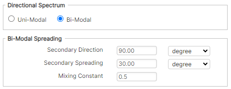
Bi-Modal – Two directional spectra are used for determining wave spreading. The following additional inputs are required to define the bi-modal spreading, as presented in Figure 4-13:

• Secondary Direction: the secondary mean direction for wave spreading relative to the pipeline (perpendicular to the pipe is 90°).
• Secondary Spreading: the secondary standard deviation of wave spreading used in the bi-modal wrapped normal spreading function.
• Mixing Constant: the value used to combine the two components of the bi-modal directional spectrum, termed a in the following:

D(\Theta)=aD_1(\Theta)+(1-a)D_2(\Theta)

D(\Theta)=aD_1(\Theta)+(1-a)D_2(\Theta)

In addition, the Level 3 calculations permit the user-specification of the number of angle divisions for wrapped normal directional spreading discretization (up to a maximum of 24), for both single and bi-modal spreading

Current Settings

Boundary Layer – Figure 3-4 presents a typical scenario where a pipeline diameter lies within the steady current boundary layer. Inclusion of current reduction due to its boundary layer can reduce the conservativeness in using free-stream current value.

The following options are provided in the software for the steady current boundary layer calculation (with the formulations below presented for a perpendicular current, for simplicity):

• User Defined: Uses the user defined current velocity as a constant value at the current angle for calculating current load.

U(z)=U_{UD}

U(z)=U_{UD}

• Logarithmic: Calculates the current load using a logarithmic relationship, given the current velocity, current angle, current reference height and seabed roughness.

\frac{U(z)}{U(z_r)} = \frac{\ln(z + z_0) – \ln(z_0)}{\ln(z_r + z_0) – \ln(z_0)}

\frac{U(z)}{U(z_r)} = \frac{\ln(z + z_0) - \ln(z_0)}{\ln(z_r + z_0) - \ln(z_0)}

• 1/7th Power: Calculates the current load using the 1/7th power law, given the current velocity, current angle and current reference height.

\frac{U(z)}{U(z_r)}=\left(\frac{z}{z_r}\right)^{\frac{1}{7}}

\frac{U(z)}{U(z_r)}=\left(\frac{z}{z_r}\right)^{\frac{1}{7}}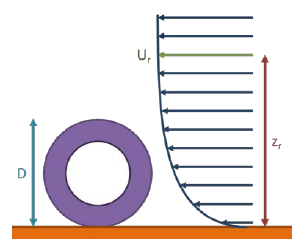

Current – The speed of the current, which acts at the reference height in the direction specified by the current angle.
Current Angle – The angle of attack at which the current acts on pipeline (perpendicular to the pipe is 90°).
Reference Height – The height above the seabed at which the current value is known (taken as the top of the boundary layer).
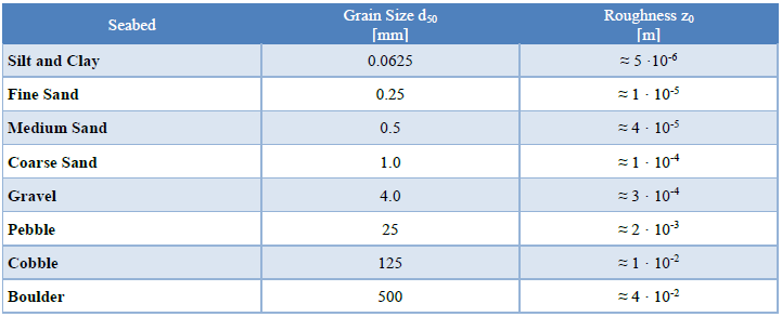
Seabed Roughness – Based on the seabed type Seabed roughness value can be input in this field. Reference can made from Table 3-1, as given in DNV-RP-F109 [2].

Applied Current Settings –
Selectable from the following options:

• Top of Pipeline: The applied current velocity is taken as the value calculated at the top of the pipe total diameter (being the pipe OD including all coatings and marine growth).
• Average over OD: The applied current velocity is taken as the average value experienced across the total OD.

Output Control Tab

This input tab controls the aspects of the printing and plotting outputs, as presented in Figure 5-13.

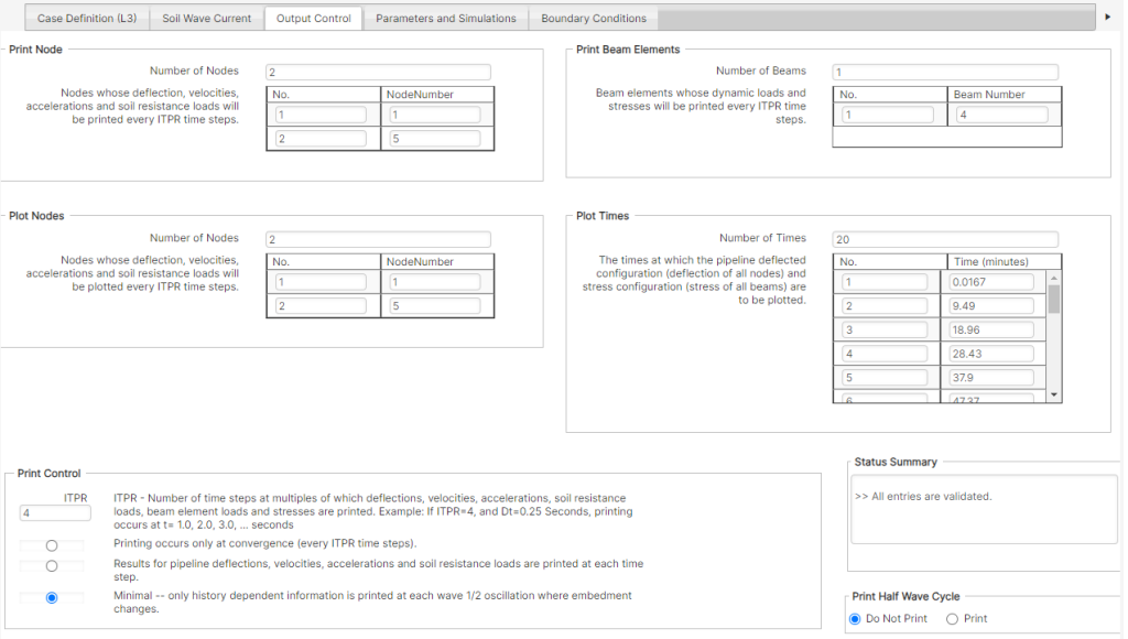
Print Nodes

What is ITPR? – A print control integer. ITPR is the number of time steps at multiples of which the deflections, velocities, accelerations, soil-resistance loads, beam element loads, and stresses are printed. Example: If ITPR = 4, and the time step interval, DT = 0.25 sec, printing occurs at t = 1.0 sec, 2.0 sec, 3.0 sec, etc.
Number of Nodes – The total number of nodes whose deflections, velocities, accelerations, and soil-resistance loads will be printed to the output file, which occurs every ITPR (a print control integer) time steps. This part of the output can be large for many time steps. For long simulation runs, it may be useful to set this value to zero to suppress this part of the output and expedite the process.
Node List – List containing the nodes numbers whose deflections, velocities, accelerations, and soil-resistance loads are to be printed to the output file, every ITPR time steps.

Print Beam Elements

Number of Beams – The total number of beam elements whose dynamic loads and stresses will be printed to the output file every ITPR time steps. This part of the output can be large for many time steps. For long simulation runs, it may be useful to set this value to zero to suppress this part of the output and expedite the process.
Beam List – List containing the beam element numbers whose dynamic loads and stresses are to be printed to the output file, every ITPR time steps.

Plot Nodes

Number of Nodes – The total number of nodes whose deflections, embedment, forces, stresses, tension and factors of safety will be written to a file every ITPR time steps, for use in plotting. This part of the output is recommended to be set greater than zero for long simulation runs whether or not plotting is planned.
Node List – List containing the nodes whose deflections, etc. will be written to a file every ITPR time steps, for use in plotting.

Plot Times

Number of Times – The total number of times at which the deflected configuration and stress configuration of the pipeline will be written to the plot file. This provides a series of instantaneous ‘snapshots’ of the pipe condition.
Time List – List containing the times at which the pipeline deflected configuration (deflection of all nodes) and stress configuration (stress of all beams) are to be written to the plot file.

Print Control

ITPR Parameter – A print control integer. ITPR is the number of time steps at multiples of which the deflections, velocities, accelerations, soil-resistance loads, beam element loads, and stresses are printed. Example: If ITPR = 4, and the time step interval, DT = 0.25 sec, printing occurs at t = 1.0 sec, 2.0 sec, 3.0 sec, etc.
Print Options – Three options are available for print output:

• Printing occurs only at convergence (every ITPR time steps).
• Results for pipeline deflections, velocities, accelerations, and soil-resistance loads are printed at each time step iteration.
• Minimal print detail (which is the default) where only history dependent information is printed at each applicable wave 1/2 oscillation where embedment changes.

Print Half Wave Cycle – Two options for print output:

• Printing is suppressed for 1/2 wave cycles.
• History dependent information is printed at each wave 1/2 oscillation.

Parameters and Simulations Tab

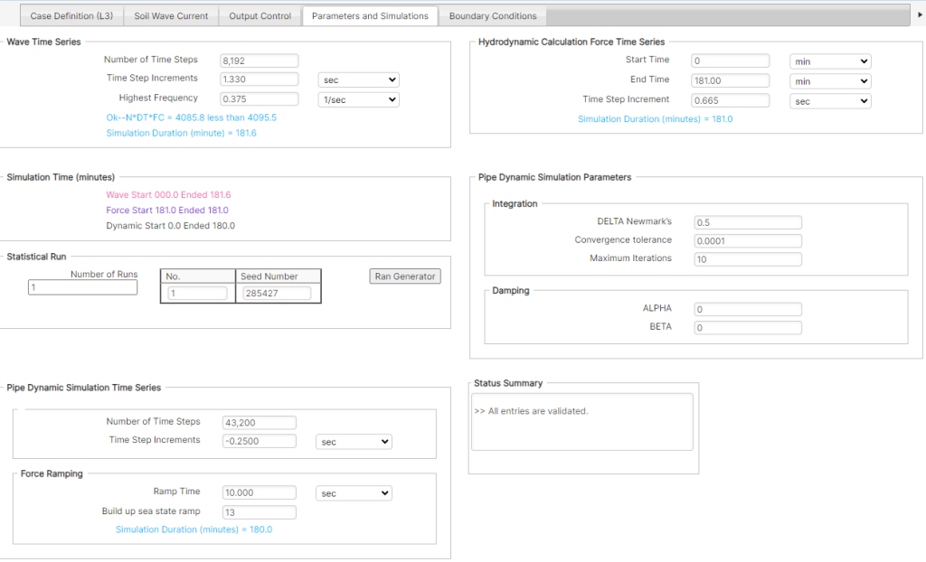
This input tab contains advanced options to control the simulation times and time steps for each analysis module, and various pipe dynamic simulation parameters, as presented in Figure 5-14.

Wave Time Series

This area defines the number of times steps (n_{time steps}), the time step increments (Δt), and the highest frequency cutoff (f_cutoff). The values of these parameters must satisfy the inequality:

n_{\text{time steps}} \cdot \Delta t \cdot f_{\text{cutoff}} < 4095.5

n_{\text{time steps}} \cdot \Delta t \cdot f_{\text{cutoff}} < 4095.5

Number of Time Steps – The number of time steps for the Random Wave Generation module, which due to the computational format should be 2 raised to a power, with 2¹⁸ (= 8192) as the maximum.
Time Step Increments – The value of the time step size for the Random Wave Generation module. Value is related to the simulation time and the number of times steps by:

\text{(Number of Time Steps)} \cdot \text{(Time Step Increments)} = \text{(Simulation Time)}\~\ n_{\text{time steps}} \cdot \Delta t = t_{\text{simulation}}

\text{(Number of Time Steps)} \cdot \text{(Time Step Increments)} = \text{(Simulation Time)}\\~\\ n_{\text{time steps}} \cdot \Delta t = t_{\text{simulation}}

Highest Frequency – The high frequency cutoff (f_cutoff below) is the highest frequency to be considered with non-negligible energy. For numerical stability, the following limit is imposed:

n_{\text{time steps}} \cdot \Delta t \cdot f_{\text{cutoff}} < 4095.5

n_{\text{time steps}} \cdot \Delta t \cdot f_{\text{cutoff}} < 4095.5

Hydrodynamic Calculation Force Time Series

Start Time – Starting time for the Hydrodynamic Force module time series.
End Time – Ending time for the Hydrodynamic Force module time series.
Time Step Increment – Time step value for Hydrodynamic Force module.

Pipe Dynamic Simulation Time Series

Number of Time Steps – Number of time steps for the Pipe Dynamic module.
Time Step Increments – Time step value (sec) used in the numerical integration (Newmark) method. If the value is specified as less than or equal to zero or left the software will select an appropriate value of 0.25 sec.

Force Ramping

Ramp Time – This is rather a numerical setup parameter The length of time over which forces are increased to their full value, in order to avoid transient effects. This ramp value is typically specified around the value of the peak wave period.
Build-up Sea State Ramp – This parameter should be specified as greater than 12 if no ramping is desired (default). Otherwise, BUP divided by 12 is the wave height ratio by which hydrodynamic forces are scaled to simulate a building sea-state. Each 20-minute BUP is incremented by 1 until BUP equals 12.

Simulation Time

This area displays the simulation duration of wave time series, hydrodynamic force calculation time series and pipe dynamic simulation time series, in minutes.

Statistical Run and Seed Numbers

In this field users can setup multiple wave seed numbers. This can be done through the Number of Runs entry (Figure 5-15). For each run, users can set specific Seed Numbers. The seed numbers can either be generated randomly by the Ran Generator button or can directly be inputted into the table by modifying the values in the relevant cells.

The generated Input/output files are also saved in a subdirectory identifiable by Id number and Seed Number as follows:

<Project Folder>\Results-Filename\Level3\Id\Seed Number

Pipe Dynamic Simulation Parameters

DELTA Newmark’s – The 𝛿𝛿 parameter of the Newmark numerical integration method. The default value is 0.5.
Maximum Iterations – Maximum number of iterations to achieve convergence at a given time step. The default value is 10. This may be increased for complex systems that fail to converge under the default number of iterations.
Convergence Tolerance – The tolerance parameter EPS, is used to check for convergence. The default value is 0.0001.
Convergence is assumed at the kth iteration when:

G^k(I) \leq EPS; \quad I = 1, 2

G^k(I) \leq EPS; \quad I = 1, 2

Where:
EPS is a very small number to determine if G(I) can be considered as small enough to be insignificant

Convergence Criteria – The convergence parameter at the k^th iteration, G^k(I), is defined as:

G^k(I) = \sqrt{\frac{\sum_{J=1}^{NC} (U^k(I,J) – U^{k-1}(I,J))^2}{NC \cdot |U_{max}(I)|}}

G^k(I) = \sqrt{\frac{\sum_{J=1}^{NC} (U^k(I,J) - U^{k-1}(I,J))^2}{NC \cdot |U_{max}(I)|}}

Where:

• I – The degree of freedom (DOF)
• NC – The number of nodes
• U^k_max – The maximum deflection at iteration k in DOF I
• U^k(I,J) – The deflection of node J in DOF I

Damping

ALPHA – The mass-proportional damping coefficient.
BETA – The stiffness-proportional damping coefficient.
ALPHA and BETA are the proportionality factors defining proportional, or classical, damping according to:

[C]=\text{ALPHA}[M]+\text{BETA}[K]

[C]=\text{ALPHA}[M]+\text{BETA}[K]

This damping may be introduced to account for structural damping.

Boundary Conditions Tab

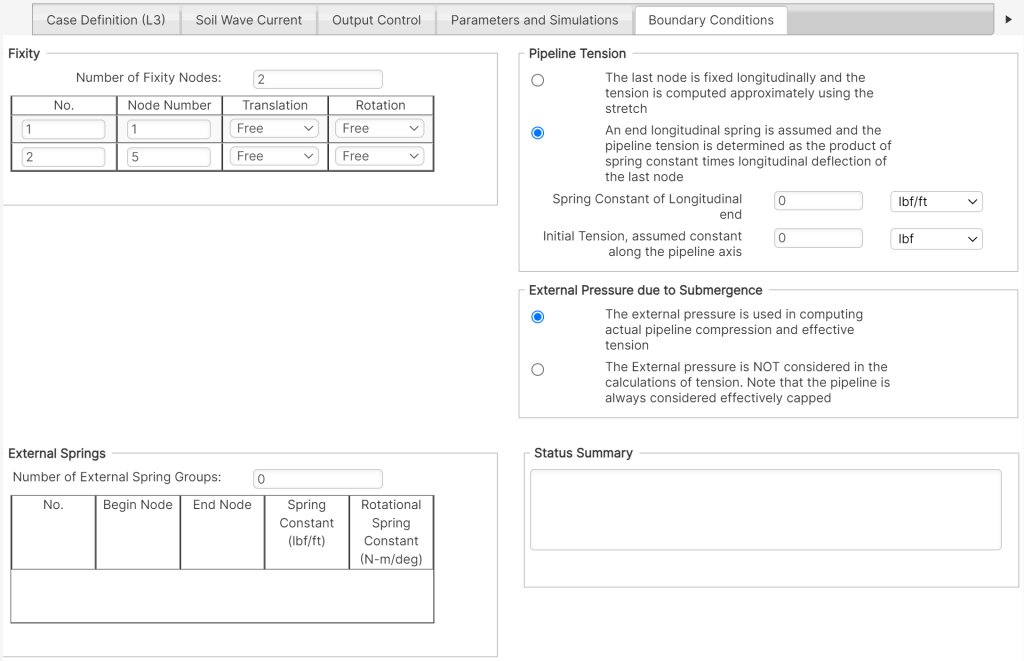
This input tab contains advanced options to control the boundary conditions: tension, fixity, external springs and the effects of external pressure, as presented in Figure 5-16.

Fixity

Number of Fixity Nodes – Number of nodes at which to specify restraints.
Node Number – The node number at which to specify restraint.
Translation – Translational fixity in the lateral and longitudinal directions, which can be set as either Free or Fixed at the specified node number.
Rotation – Rotational fixity in the horizontal plane (about the vertical Z-axis), which can be set as either Free or Fixed at the specified node number.

External Springs

Number of External Springs Groups – The specification of external springs can be varied over the length of the pipeline, up to a maximum of ten external spring groups.
Begin Node – Starting node for the external spring group.
End Node – Ending node for the external spring group.

Note: If the ending node number is zero or blank, springs are added at the beginning node number only. The nodal increment from beginning node to ending node is 1.

Spring Constant – Translational spring constant of the springs applied to nodes of the current external spring group, applicable in degree of freedom 1 (lateral direction).
Rotational Spring Constant – Rotational spring constant of the springs applied to nodes of the current external spring group, applicable in the rotational degree of freedom in the horizontal plane (about the vertical Z-axis).

Pipeline Tension

Pipeline Tension Option – Two options are selectable for the calculation of pipeline tension:

• The last node is fixed longitudinally and the tension is computed approximately using the stretch.
• A longitudinal spring is assumed to act at the end, and the pipeline tension is determined as the product of spring constant multiplied by the longitudinal deflection of the last node.

Spring Constant of Longitudinal End – The spring constant of the optional longitudinal spring at the last node of the pipeline.
Initial Tension – Initial pipeline tension, which is assumed constant along the pipe longitudinal axis.

External Pressure due to Submergence

These options allow the software to either consider or ignore the effect of external hydrostatic pressure:

• The external pressure is used in computing actual pipeline compression and effective tension (default).
• The external pressure is not considered in the calculations of tension.

Note: That the pipeline is always considered as effectively capped.

Level 3 Reports

The primary outputs of the Level 3 time-domain analysis are presented through various reports and plots. Generation of reports for the Level 3 analysis is facilitated by the Reports drop down menu, as presented in Figure 5-17. Due to the size of the output data, the PDF reports are not generated automatically after the analysis is completed. Instead, each report is generated whenever the user chooses an item in the menu

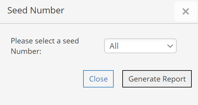
By clicking on each of report options, the user can select which seed number to report through a secondary dropdown list as illustrated in Figure 5-18.

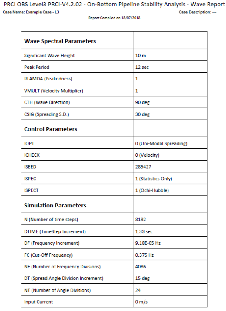
Wave Report

This report displays the wave related parameters calculated by the software, along with some key user input values, as presented in Figure 5-19. The report can be found as L3_Wave_Report.pdf in <Project Folder>\Results-Filename\Level3\Id\Seed Number.

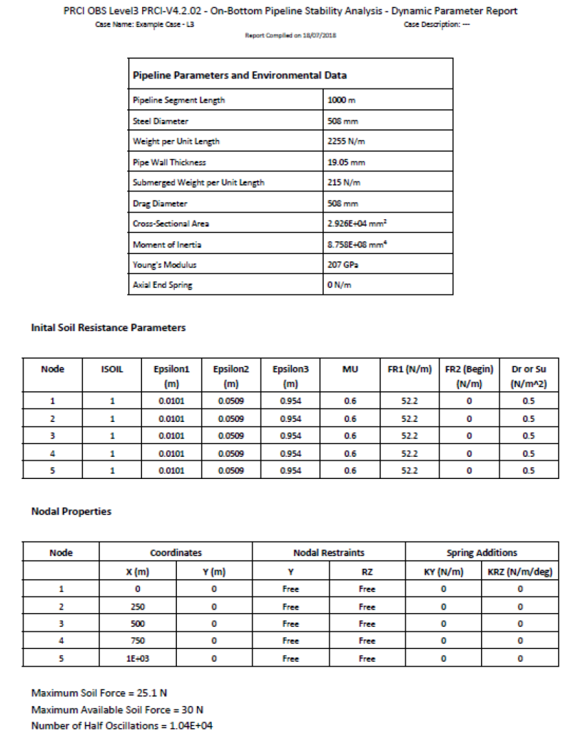
Dynamic Parameters Report

This report displays soil resistance parameters and other data calculated by the software, as presented in Figure 5-20. The report can be found as L3_DynParams_Report.pdf in <Project Folder>\Results-Filename\Level3\Id\Seed Number

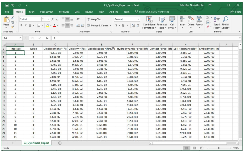
Dynamic Nodal Report

This report displays nodal deflections, velocities, accelerations and seabed loads calculated by the software. The report is generated in the CSV form, named as L3_DynNodal_Report.csv and saved in <Project Folder>\Results-Filename\Level3\Id\Seed Number

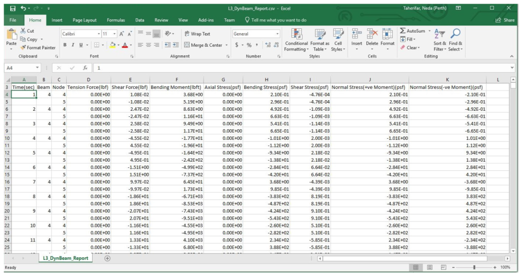
Dynamic Beam Report

This report displays the loads and stresses calculated by the software, on the specified beam elements, as presented in Figure 5-22. The report is generated in the CSV form, named as L3_DynBeam_Report.csv and saved in <Project Folder>\Results-Filename\Level3\Id\Seed Number

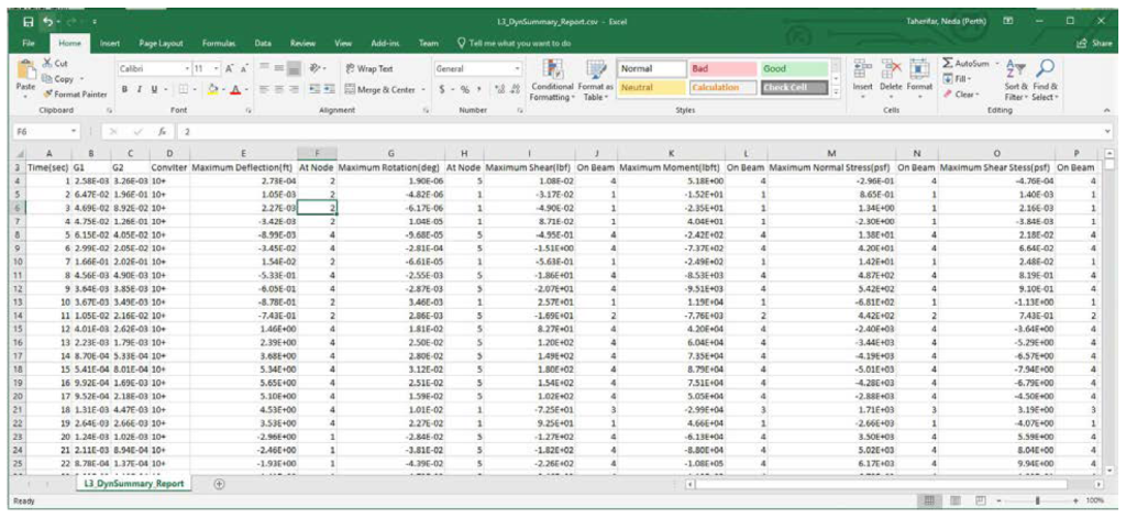
Dynamic Summary Report

This report displays the summary of convergence and maximum values of the dynamic analysis, as presented in Figure 5-23. The report is generated in the CSV form, named as L3_DynSummary_Report.csv and saved in <Project Folder>\Results-Filename\Level3\Id\Seed Number

Statistical Summary Report

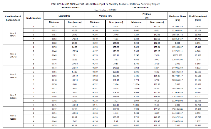
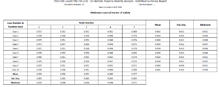
This report displays the summary of the multiple time domain analysis runs and statistical information on the output parameters, as presented in Figure 5-24 and Figure 5-25. The report can be found as L3_Stats Summay_Report.pdf in <Project Folder>\Results-Filename\Level3\Id\Seed Number

Level 3 Plots

Control of the generation, viewing and printing of output data plots for the Level 3 analyses is facilitated by the options in the Plots drop down list, as presented in Figure 5-26. Each of the plot menu items opens a window to display the selected plot, with various view options.

Velocity Plot

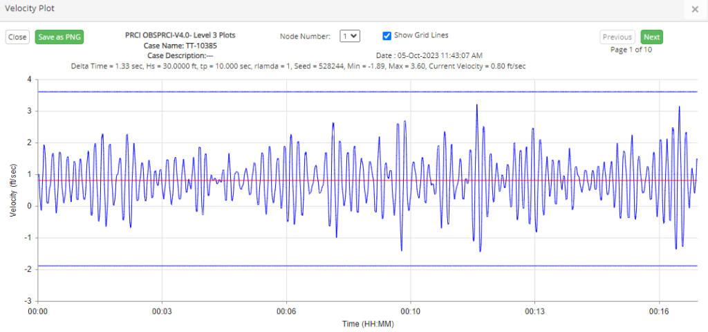
Displays the velocity time series output from the random wave generation module, as presented in Figure 5-27. The line in the middle of the plot indicates the magnitude of the contribution of the steady current velocity. The plot window will automatically scale and break the plot up into a number of pages to ensure adequate resolution of the time series (note if resolution is not desirable the same data may be plotted through the Pipeline Dynamic Plot menu item).

The plot window has button options to Close the plot window, view the Previous and Next page of the time series plot, and Save as PNG the current page of the time series plot.

The user can choose the node number as well as the seed number at which the data to be displayed.

Hydrodynamic Plot

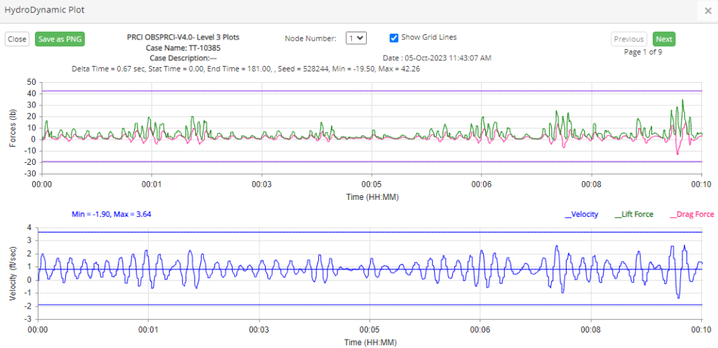
Displays the raw (static pipe) lift and drag forces output from the hydrodynamic force module at top half of the page and a velocity time series plot at the bottom half of the page, as presented in Figure 5-28. This plot is useful to illustrate the velocities and the resultant hydrodynamic forces. The plot window will automatically scale and break the plot up into a number of pages to ensure adequate resolution of the time series (note if resolution is not desirable the same data may be plotted through the Pipeline Dynamic Plot menu item).

The plot window has button options to Close the plot window, view the Previous and Next page of the time series plot, and Save as PNG the current page of the time series plot.

The user can choose the node number as well as the seed number at which the data to be displayed.

Pipeline Dynamic Plot

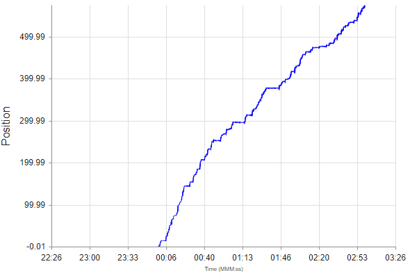
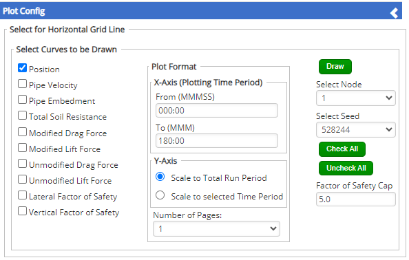
Displays a dynamic plot selection window that enables more detailed customization of plot generation, as presented in Figure 5-29. The available controls include the selection of the data curves to be plotted, the scope (time series) and scaling (magnitude) of the plot, the desired number of pages for splitting of the plot, the node and the seed number for which the data is to be plotted, and a factor of safety cap.

Select Curves to be Drawn

This area contains a menu to select which data time series are to be drawn including Position, Fluid Velocity, Pipe Embedment, Total Soil Resistance, Modified (with pipe moving) Drag and Lift Forces, Unmodified (static pipe) Drag and Lift Forces, and the Lateral and Vertical Factors of Safety. The checkboxes allow one or more curves to be drawn simultaneously on the same plot.

Plot Format – This area includes the following inputs:

• X-Axis (Plotting Time Period): Specifies the start and end times for the plot (in MMM:SS format). These values default to the entire time series.
• Y-Axis: Controls the automatic y-axis scaling to either the maximum and minimum of the entire time series or the maximum and minimum of the selected time interval.
• Number of Pages: Sets the number of pages the selected time series plot is split over.

DRAW Button – Generates the plot and opens the dynamic plot window to view and print the resulting plot selection.
Select Node – Allows specification of the number of the node at which to display the time series.
Select Seed – Allows specification of the seed at which to display the time series.
Check All and Uncheck All Buttons – Selects and de-selects (respectively) all data time series to be plotted.
Factor of Safety Cap – Factor of safety get large as the lift and drag forces reverse (and when force is zero, the instantaneous factor of safety goes to infinity). Thus, the user can specify a cap on the maximum value of factor of safety to be displayed to obtain the desired resolution of the data.
The factors of safety are defined as:

FOS_{\text{lateral}} = \frac{\text{Soil Resistance}}{\text{Modified Drag Force}} \~\ FOS_{\text{vertical}} = \frac{\text{Submerged Weight}}{\text{Modified Lift Force}}

FOS_{\text{lateral}} = \frac{\text{Soil Resistance}}{\text{Modified Drag Force}} \\~\\ FOS_{\text{vertical}} = \frac{\text{Submerged Weight}}{\text{Modified Lift Force}}

Stress and Deflected Plot

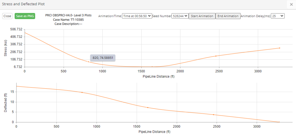
This plot displays normal stress (bending + axial) and deflected configuration output data, as presented in Figure 5-30. These data series are snapshots of the instantaneous stress and deflected position of the entire model length at a selected time. These times are specified in the Output Control input tab, under the Plot Times selection.

These configurations can be either displayed as an animated series (where the display increments through the plots to create a “movie”), or as individual snapshots. The options for animation and static display times are selectable in an input form at the top of the page.

Select Animation or a Time Period (HH:MM:SS)

This dropdown list enables selection of either Animation or of one of the specific time snapshots. If animation is chosen then by clicking on Start Animation button, the stress and deflected animation loop can be seen. For the specific time snapshots, the window will display the static plots for the chosen time period, which can be saved as PNG using the Save as PNG button.

Seed Number – Through the dropdown list a Seed Number can be selected in order to observe the corresponding results.
Start Animation – This button will begin the animation if the Animation option is selected.
Animation Delay (ms) – The rate of the animation can be controlled from 25 (very fast) to 3200 (slower).

Level 3 Additional Technical Description

Random Wave Generation

Directional Wave Spectra Model – The directional wave (sea surface) spectral density, S(f,Θ) is a function of frequency, f, and direction, Θ; and is expressed as the product of two parametric quantities, frequency spectral density, S(f), and D(Θ), the directional spreading function:

S(f,\Theta)=S(f)\cdot D(\Theta)

S(f,\Theta)=S(f)\cdot D(\Theta)

Where:

• S(f) – The sea surface frequency spectral density
• D(Θ) – The spreading function at frequency, f
• ∫₀^2𝜋 𝐷(𝛩)𝑑𝛩 = 1.0, by definition

This involves a substantial simplification because S(f,Θ) is taken as separable (i.e. the spreading function, D(Θ), is actually only a function of Θ and not of f) over the frequencies where substantial wave energy is present. This assumption is reasonable for wave periods affecting submarine pipelines.

Frequency Spectral Density – A three parameter generalization of the Pierson-Moskowitz-Bretschneider formula [8] is used for S(f), and the wrapped-normal directional density ([8], [9]) is used for D(Θ). This characterizes the sea surface with five input parameters. The original Ochi-Hubble formulation contains six parameters. However, the high frequency component contributes little to the pipeline motion and has, therefore, been deleted, eliminating three terms.

The formulation of the three-parameter spectral density developed by Ochi and Hubble is expressed as a one-sided function of radian frequency. This formula may be modified to the two-sided function of cycles-per-second frequency, for -∞ < f < ∞, to obtain:

S(f)=\frac{2\left( \frac{(4\lambda+1)f_0^4}{4} \right)^\lambda \sigma^2e^{\frac{-(4\lambda+1)\left(\frac{f_0}{f} \right)^4}{4}} }{\Gamma(\lambda)|f|^{4\lambda+1}}

S(f)=\frac{2\left( \frac{(4\lambda+1)f_0^4}{4} \right)^\lambda \sigma^2e^{\frac{-(4\lambda+1)\left(\frac{f_0}{f} \right)^4}{4}}   }{\Gamma(\lambda)|f|^{4\lambda+1}}

Where Γ(λ) is the complete gamma function. By the definition of a two-sided spectral density, the variance of the sea surface elevations is given by:

\sigma^2 = \int_{-\infty}^{\infty} S(f) df = 2 \int_{0}^{\infty} S(f) df

\sigma^2 = \int_{-\infty}^{\infty} S(f) df = 2 \int_{0}^{\infty} S(f) df

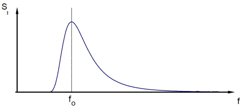
The spectral function has a maximum (denoted by S) at f = f₀. This may be verified by differentiating the spectra and setting the derivative equal to zero. Consequently, an expression for S may be obtained by setting f equal to f₀:

S = \frac{2\left(\frac{4\lambda+1}{4}\right)^\lambda}{\Gamma(\lambda)|f_0|} \sigma^2 e^{\frac{-(4\lambda+1)}{4}}

S = \frac{2\left(\frac{4\lambda+1}{4}\right)^\lambda}{\Gamma(\lambda)|f_0|}  \sigma^2 e^{\frac{-(4\lambda+1)}{4}}

This formula depends on three parameters, f₀, σ², and λ. The parameters f₀ and σ² have direct geometric interpretations. The parameter f₀ is the frequency at which the spectrum reaches its maxima. The variance, σ², is the area under the spectral density in (-∞, ∞) or twice the area under S(f) in (0, ∞). This leaves λ as a fitting parameter to force the function to have maximum height of S.

Lambda, λ, is a mathematical parameter which measures the width of the spectral density function, S(f), and is a function of another more intuitive (or geometric) parameter called the effective width of the spectrum. Consider the diagram in Figure 5-31. The area under the spectral density from (0, ∞) is σ²/2. The height of the spectra at f=f₀ is S(f₀). The effective width is defined to be the width of the rectangle which is S(f₀) tall and which equals the area under S(f).

The Ochi-Hubble function can represent fairly well many spectral shapes. Very narrow spectra (small δ) give large values of λ. Very broad spectra (large δ) give small values of λ. If λ = 1, the function becomes a form of the Pierson-Moskowitz-Bretschneider spectral density. If λ = 1.664, the function becomes a form of the JONSWAP spectrum.

Ochi-Hubble Wave Spectrum in Level 3 Module (Double Sided) – The Ochi-Hubble spectral function is plotted in Figure 5-31 and given by:

S_\eta(f)=\frac{2\left( \frac{(4\lambda+1)f_0^4}{4} \right)^\lambda \sigma^2e^{\frac{-(4\lambda+1)\left(\frac{f_0}{f} \right)^4}{4}} }{\Gamma(\lambda)|f|^{4\lambda+1}}

S_\eta(f)=\frac{2\left( \frac{(4\lambda+1)f_0^4}{4} \right)^\lambda \sigma^2e^{\frac{-(4\lambda+1)\left(\frac{f_0}{f} \right)^4}{4}}   }{\Gamma(\lambda)|f|^{4\lambda+1}}

Where:

• Γ(λ) – The Gamma Function
• 𝜎² = 2∫₀^∞𝑆_𝜂(𝑓)𝑑𝑓 – The variance of sea surface elevation
• σ – The standard deviation of water surface elevation
• H_s = 4σ is the significant wave height
• f₀ – The peak frequency
• T_p = 1/f₀ is the peak period

Directional Spreading Function – Various spreading function formulas such as the von Mises, the generalized cosine-squared [11], and the wrapped-normal function can all represent, with about the same accuracy, the spreading function for waves where the function is unimodal and roughly symmetric. Thus, it appears reasonable to use the formula which is most tractable mathematically. The wrapped-normal matches this criterion and is used in the current version of the Level 3 module.

The wrapped-normal formula may be expressed in two mathematically equivalent forms:

D(\Theta)=\frac{1}{2\pi}+ \sum_{n=1}^{\infty} e^{\frac{-n^2 \sigma_{D}^2}{2}}\cos (\Theta-\Theta_0)\~\= \sum_{n=1}^{\infty}\frac{\exp\left(\frac{\left(-\frac{1}{2}(\theta-\theta_0)-2\pi k \right)^2}{\sigma^2_D} \right)}{\sqrt{2\pi}\cdot \sigma_D}

D(\Theta)=\frac{1}{2\pi}+ \sum_{n=1}^{\infty} e^{\frac{-n^2 \sigma_{D}^2}{2}}\cos (\Theta-\Theta_0)\\~\\=  \sum_{n=1}^{\infty}\frac{\exp\left(\frac{\left(-\frac{1}{2}(\theta-\theta_0)-2\pi k   \right)^2}{\sigma^2_D}  \right)}{\sqrt{2\pi}\cdot \sigma_D}

If σ_D < π/3, as is usually the case for storm waves, the second formula (in the exponential form) will have only one term in the summation which is not essentially zero. Thus, the spreading function would then become:

D(\Theta)=\frac{e^{-\frac{1}{2}}\left( \frac{\Theta-\Theta_0}{\sigma_D}\right)^2}{\sqrt{2\pi \sigma_D}}

D(\Theta)=\frac{e^{-\frac{1}{2}}\left( \frac{\Theta-\Theta_0}{\sigma_D}\right)^2}{\sqrt{2\pi \sigma_D}}

This is providing Θ is restricted to the interval (Θ₀-π, Θ₀+π). The wave energy is being spread over the various angles by what is functionally equivalent to a normal probability density with standard deviation, σ_D.

In the unimodal option (default), the wrapped normal spreading function is used for D(Θ). The vector of directional spreading values are computed from parametric input based on a central direction, H₀, (direction toward which the waves are traveling) and a directional standard deviation, σ_D. The standard deviation can be directly compared with the corresponding parameter in the usual normal probability density. That is about 2/3 of the energy is contained between Θ₀-σ_D and Θ₀+σ_D.

The bi-modal option (an advanced feature) is very similar to the unimodal option, except that two wrapped normal spreading functions at each frequency are used.

D(\Theta)=aD_1(\Theta)+(1-a)D_2(\Theta)

D(\Theta)=aD_1(\Theta)+(1-a)D_2(\Theta)

Here “a” is a selected constant, 0 < a < 1, and D_j(Θ) are each wrapped normal spreading functions with their own sets of Θ₀ and σ_D values.

Input Parameters –

The values of S(f) and D(Θ) are developed in the software as two vectors NF and NT long, respectively. Here NF denotes number of frequencies and NT is the number of theta values. Frequency is expressed in cycles per second, or Hertz, and Θ is in degrees. The frequency increment is DF, representing Δf, and the angle increment is DR, standing for ΔΘ.

The number of terms in the simulated wave time sequence is N. As an advanced option, this value can input directly (rather than generated by the pre-processor) and must be an integer power of 2, (i.e. N=2^K). If not, the value is rounded down to the next lowest integer power of 2.

The time increment, DT, can also be directly input, and since DT=1.0/(N*DF); this also fixes the frequency internal, DF. The aforementioned relation is required by the fast Fourier transform algorithm used in the simulation.

The cut-off frequency, FC, can also be input. Given the cut-off frequency, FC, and the frequency interval, DF, the number of frequencies, NF is defined.

NF=DF \cdot FC

NF=DF \cdot FC

The value of NF must satisfy two requirements. The values of NF and DF must be selected so that:

1. S(F,Θ) is negligible (close to zero) for f > NF*DF, and
2. NF must be less than half of N, where N is the length, or number of terms, in the time series of wave properties being simulated.

For stability of the fast Fourier transform applied in the wave generation module, the product of M, DT and FC must be less than 4095.5 to ensure convergence. This is satisfied automatically with values chosen by the pre-processor, but must be enforced if the values are input.

As an advanced option, the number of theta values, DT, can be directly input. The values of DT and NT are chosen so that NT*DT is a full circle, 360°. The default option sets DT to the maximum value allowed by the software, 24. Other input parameters are covered in sufficient detail in the input instructions.

Hydrodynamic Force Calculation

Decomposition of Irregular Waves – By decomposing a time series of bottom wave velocities in irregular waves into zero-upcrossing and zero-downcrossing half-wave cycles it is possible to define local wave parameters, such as the KC-number and the current ratio, a, see Figure 5-32. The half-wave cycle is by no means sinusoidal. It is, however, treated as a regular wave with an amplitude equal to the maximum absolute value of the observed velocity during the corresponding upcrossing or downcrossing half-wave cycle, and with a wave period equal to twice the half-wave period.

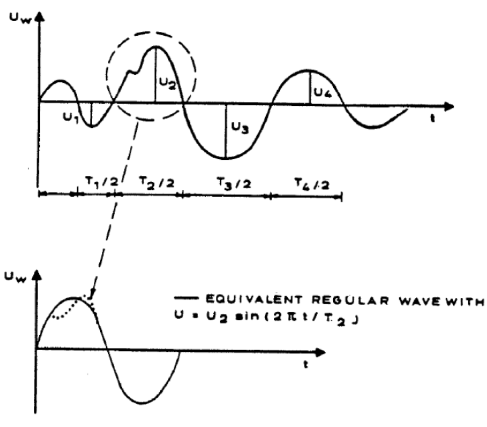
The non-dimensional wave parameters are thus calculated as:

KC_1 = \frac{2 \cdot |U_{w1}| \cdot \frac{T_1}{2}}{D}, \quad \alpha_1 = \frac{U_c}{|U_{w1}|} \[10pt] KC_2 = \frac{2 \cdot |U_{w2}| \cdot \frac{T_2}{2}}{D}, \quad \alpha_2 = \frac{U_c}{|U_{w2}|} \[10pt] \dots \[10pt] KC_n = \frac{2 \cdot |U_{wn}| \cdot \frac{T_n}{2}}{D}, \quad \alpha_n = \frac{U_c}{|U_{wn}|}

KC_1 = \frac{2 \cdot |U_{w1}| \cdot \frac{T_1}{2}}{D}, \quad \alpha_1 = \frac{U_c}{|U_{w1}|} \\[10pt] KC_2 = \frac{2 \cdot |U_{w2}| \cdot \frac{T_2}{2}}{D}, \quad \alpha_2 = \frac{U_c}{|U_{w2}|} \\[10pt] \dots \\[10pt] KC_n = \frac{2 \cdot |U_{wn}| \cdot \frac{T_n}{2}}{D}, \quad \alpha_n = \frac{U_c}{|U_{wn}|}

Where n is the total number of half-wave cycles, U_w the maximum wave velocity, T/2 the half-wave period, and U_c is the steady current, which is assumed constant for all n. The steady current, U_c applied when calculating the local current ratio, α, is the mean current over one pipe diameter. This value may either be given directly (default) or it may be calculated based on an assumed logarithmic velocity profile. In the present version a procedure is included which is based on the calculations performed by the Current Complex Model (PRCI PR-169-186 [12]). In this case the bottom friction must be given as input in terms of a drag coefficient in addition to the steady current at a reference level 1 m above the sea bed.

Force Calculation – The hydrodynamic forces during the first part of half period No. 2 are mainly determined by the reversal of the wake created in the previous half period, No. 1.

The properties of this wake are determined by the parameters associated with half period No. 1, and the forces in the first part of half period No. 2 are then those associated with a regular wave corresponding to half wave No. 1. For the remainder of half period No. 2, the flow (and hence the forces) correspond to those associated with the regular wave defined by the parameters of half period No. 2, i.e.:

KC_2=U_2\cdot\frac{T_2}{D}\:\text{and}\:\alpha_2=\frac{U_c}{U_2}

KC_2=U_2\cdot\frac{T_2}{D}\:\text{and}\:\alpha_2=\frac{U_c}{U_2}

In PR-170-185 [6] it was found that the Fourier decomposition method was superior in predicting the hydrodynamic forces associated with regular waves (with or without steady current). This method is therefore applied to calculate the forces corresponding to the single half regular waves. The force model reads in analytical format:

t’ < t < t’ + 0.25 \cdot \frac{T_2}{2}: \quad F = \frac{1}{2} \cdot\rho \cdot D \cdot U_1^2 \left( C_{01} + \sum_{1}^{5} C_{n1} \cdot \cos(n(\omega_2 t + \phi_{n1})) \right) \[10pt] t’ + 0.25 \cdot \frac{T_2}{2} < t < t’ + \frac{T_2}{2}: \quad F = \frac{1}{2} \cdot \rho \cdot D \cdot U_2^2 \left( C_{02} + \sum_{1}^{5} C_{n2} \cdot \cos(n(\omega_2 t + \phi_{n2})) \right)

t' < t < t' + 0.25 \cdot \frac{T_2}{2}: \quad F = \frac{1}{2} \cdot\rho \cdot D \cdot U_1^2 \left( C_{01} + \sum_{1}^{5} C_{n1} \cdot \cos(n(\omega_2 t + \phi_{n1})) \right) \\[10pt] t' + 0.25 \cdot \frac{T_2}{2} < t < t' + \frac{T_2}{2}: \quad F = \frac{1}{2} \cdot \rho \cdot D \cdot U_2^2 \left( C_{02} + \sum_{1}^{5} C_{n2} \cdot \cos(n(\omega_2 t + \phi_{n2})) \right)

Here t’ is the time for the zero-crossing at the start of half period No. 2. C₀₁, C₁₁ … C₅₁, and Φ₀₁, Φ₁₁ … Φ₅₁ are the Fourier coefficients and phases related to the force associated with the regular wave defined by KC₁ and α₁. Similarly, C₀₂, C₁₂ … C₅₂ and Φ₁₂, Φ₂₂ … Φ₅₂ are those associated with the force determined by the second half wave. ω₂ is the cyclic frequency of the half period No. 2, i.e. ω₂ = 2π/T₂.

In summary, the forces in the half period No. 2 are in the first 25 percent of the time found as those associated with a regular wave flow defined by the parameters of the previous half period (No. 1) and for the latter 75 percent of the time by the forces associated with the present half wave (No. 2).

The equations given above apply to the in-line drag force and the lift force components, with different sets of coefficients and phases. The total in-line force is found by adding the inertia term,

F_I=\frac{\pi}{4}\cdot \rho\cdot D^2\cdot C_M\cdot a(t), \,\text{taking}\,\,C_M=3.29

F_I=\frac{\pi}{4}\cdot \rho\cdot D^2\cdot C_M\cdot a(t), \,\text{taking}\,\,C_M=3.29

In the PR-170-185 [6] project it was demonstrated that this force prediction model yields accurate time series for in-line as well as lift forces.

Data Base – In the present version, the data base contains Fourier coefficients for relative pipe roughness, k/d = 10^-3, 10^-2 and 5·10^-2 and for test conditions as outlined in Table 5-1.

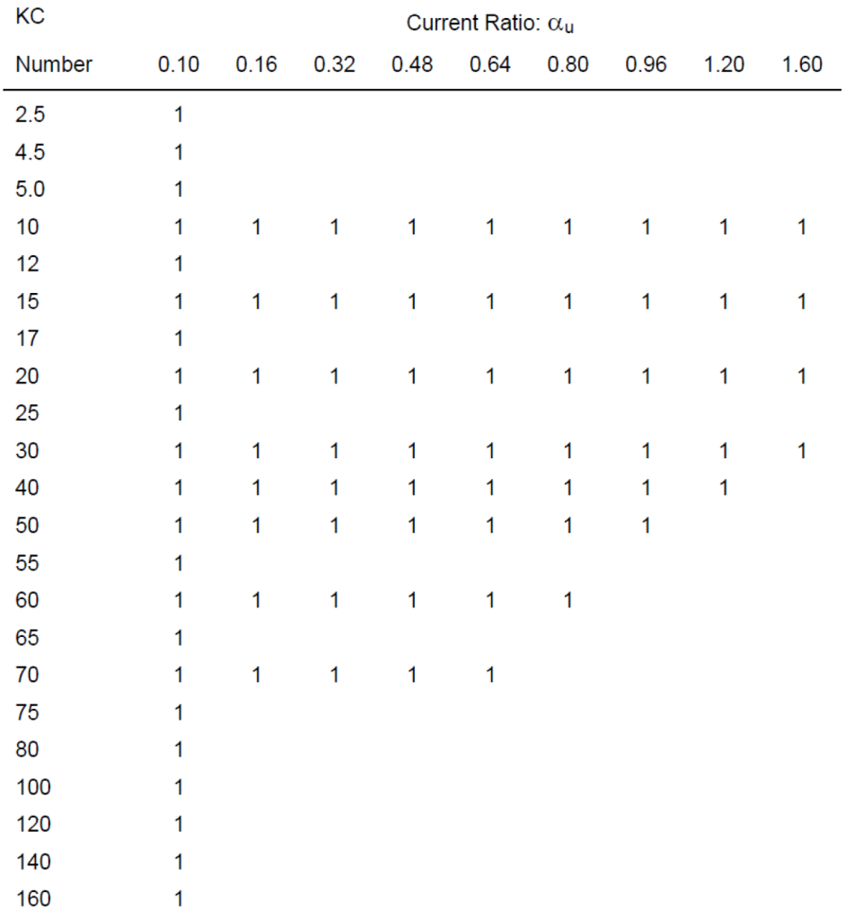
The content of the data base is illustrated in Figure 5-33 below, showing a plot of the Fourier coefficients and phases.

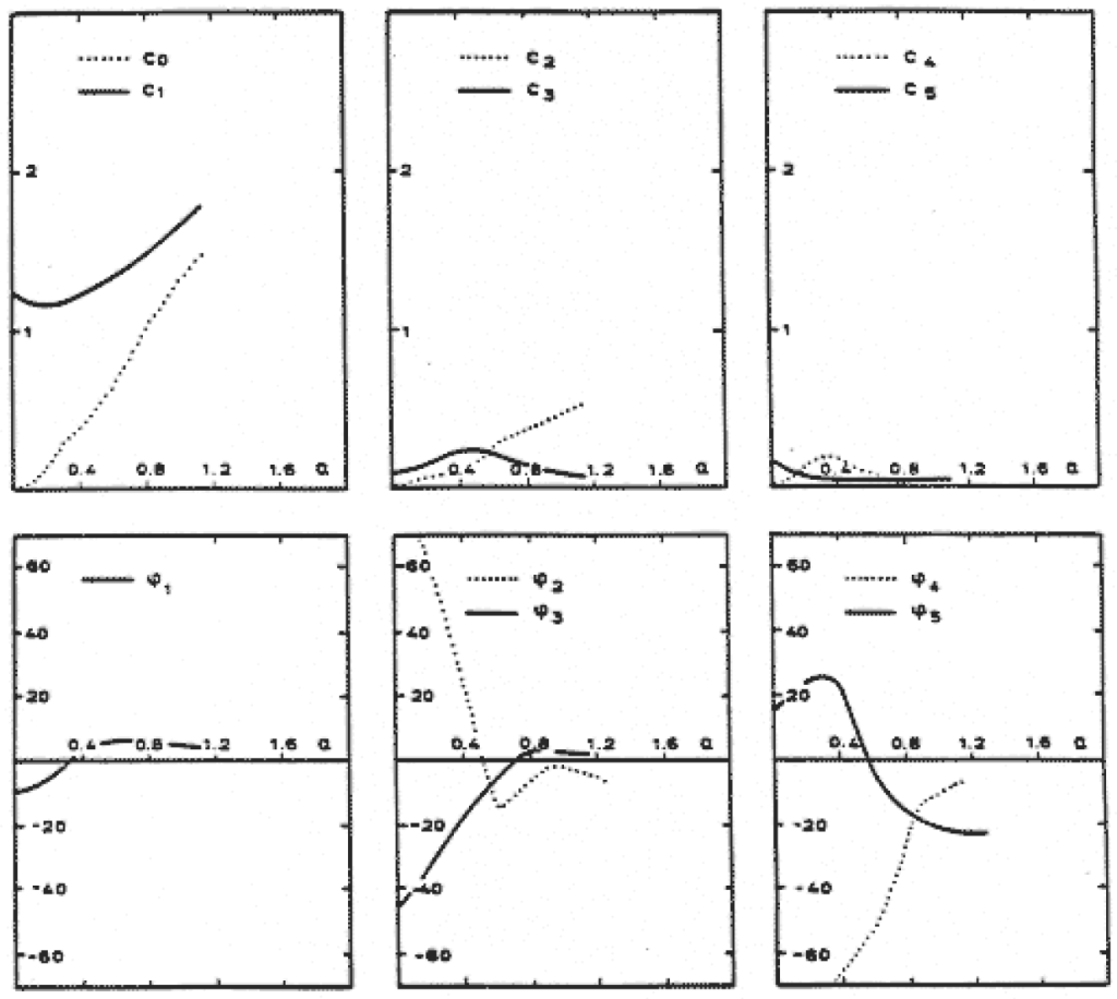
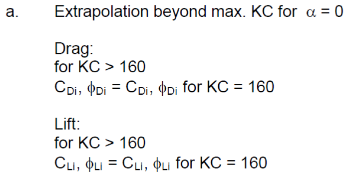
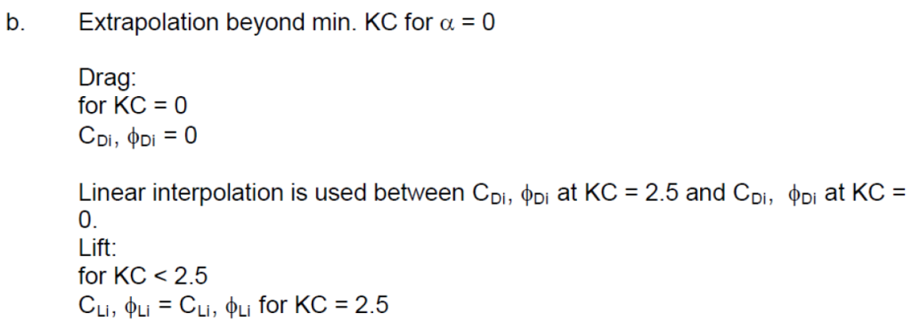
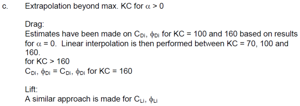
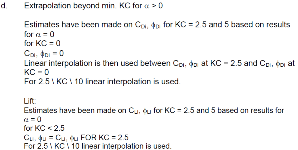
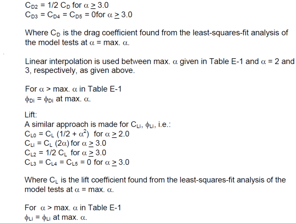
Within the ranges listed in Table 5-1, linear interpolation has been applied. For local KC-numbers and current ratios beyond these ranges various extrapolation routines have been adopted as follows:

Pipe Dynamics Simulation

General – Basically, WINDYNA solves the Euler-Bernoulli equation for bending of a uniform beam under tension. Finite beam elements (with cubic shape functions) are used to model the pipeline, and the Newmark numerical integration scheme is use to integrate the non-linear equations of motion. At each time step an iterative procedure is used to satisfy dynamic equilibrium.

Specifically, the Euler-Bernoulli equation:

EIu” – T_{e}u’ + C\dot{u} + \”{m} = q_{a}(x,t) + q_{s}(s,t) + q_{h}(x,t)

EIu'' - T_{e}u' + C\dot{u} + \"{m} = q_{a}(x,t) + q_{s}(s,t) + q_{h}(x,t)

is reduced to:

[M]{U}+[C]{U}+[K]{U}={R}

[M]\{U\}+[C]\{U\}+[K]\{U\}=\{R\}

Where:

• [M] is the inertia matrix
• [C] is the proportional damping matrix
• [K] is the stiffness matrix
• {U} is the vector of nodal deflections
• {R} is the resultant load vector

And solved at each incremented time step using the Newmark method:

[K]{U_{t+Dt}}={R_{t+Dt}}

[K]\{U_{t+Dt}\}=\{R_{t+Dt}\}

Where:

• [K_e] is the effective stiffness matrix = [K] + a₁ [M] + a₂ [C]
• {U_t+Dt} is the vector of nodal deflections at time t+Dt
• {R_t+Dt} is the resultant load vector at time t+Dt
• a₁, a₂ are integration constants

An iterative procedure known as “Successive substitution” is used at each time step until convergence is reached at each time step.

[K_e^i] {U^{i+1}} = {R^i}

[K_e^i] \{U^{i+1}\} = \{R^i\}

Where the superscript i denotes the “i”th iteration.

The software module was originally developed during project PR-175-420 [13], and the details of the module can be found in the final report for that project. The basic programming is the same; however, many modifications regarding the hydrodynamic and soil models have been incorporated.

Convergence Criteria – The convergence parameter at the k^th iteration, G^k(I), is defined as:

G^k(I) = \sqrt{\frac{\sum_{J=1}^{NC} (U^k(I,J) – U^{k-1}(I,J))^2}{NC \cdot |U_{max}(I)|}}

G^k(I) = \sqrt{\frac{\sum_{J=1}^{NC} (U^k(I,J) - U^{k-1}(I,J))^2}{NC \cdot |U_{max}(I)|}}

Where:

• I is the degree of freedom (DOF)
• NC is the number of nodes
• U^k_max is the maximum deflection at iteration k in DOF I
• U^k(I,J) is the deflection of node J in DOF I

Convergence is assumed when:

G^k(I) \leq EPS; \quad I = 1, 2

G^k(I) \leq EPS; \quad I = 1, 2

Where:

• EPS is a very small number to determine if G(I) can be considered as small enough to be insignificant.

References

1. Verley, R. L. P. and Lund, K. M. A Soil Resistance Model for Pipelines Placed on Clay Soils, OMAE – Volume 5, 1995
2. DNV-RP-F109, On-Bottom Stability Design of Submarine Pipelines, Det Norske Veritas, Nov-2011
3. Ochi, M. K. Hubble, E.N. Six-parameter wave spectra, Proceedings 15th International Conference on Coastal Engineering, Honolulu, 1976
4. DNV-OS-F101, Submarine Pipeline Systems, Det Norske Veritas, Oct-2013
5. On-Bottom Stability in Deep Waters Note, Det Norske Veritas
6. Catalog No. L51522e, PR-170-185, Hydrodynamic Forces on Pipelines: Model Tests, Prepared for PRCI by the Danish Hydraulic Institute, Dec-1986
7. PR-170-716, Hydrodynamic Forces Acting on a Pipeline in an Open Trench, Prepared for PRCI by the Danish Hydraulic Institute, Jan-1988
8. Ochi, M. K. and Hubble, E.N. Six-Parameter Wave Spectra, Proceedings 15th International Conference on Coastal Engineering, Honolulu, 1976
9. Mardia, K. V., Statistics of Directional Data. London: Academic Press, 1972
10. Borgman L.E., Directional Wave Spectra from Wave Sensors. In: Earle M.D., Malahoff A. (eds) Ocean Wave Climate. Marine Science, vol 8. Springer, Boston, MA, 1979
11. Mardia, K.V., Some properties of clasical multi-dimesional scaling,Communications in Statistics – Theory and Methods, 1978
12. PR-169-186
13. PR-175-420
14. Catalog No. L51570e, Contract PR-194-719, Energy Based Pipe-Soil Interaction Models, PRCI, June 1988
15. PR-162-157
16. PRCI Project PR-178-04405, Submarine Pipeline On-Bottom Stability Volume 1: Analysis and Design Guidelines, Kellogg Brown & Root, Inc., Dec-2008
17. PRCI Project PR-178-04405, Submarine Pipeline On-Bottom Stability Volume 2: Analysis and Design Guidelines, Kellogg Brown & Root, Inc., Dec-2008
18. Abdolmaleki, K. and Gregory, C. J., Performance of Pipe-Soil Interaction Models in a Quasi-Dynamic Approach to Pipeline Stability Analysis, OMAE-77988, 2018, Spain
19. Jacobsen, V., Bryndum, M.B., and Bonde, C., “Fluid Loads on Pipelines: Sheltered or Sliding,” Proc. 21st Offshore Technology Conference, Paper No. OTC 6056, Houston, 1989

FAQ