Surge Analysis – Water Hammer

Introduction

These equations are primarily used for calculating pressure drops and flow rates. However, a modified Reynolds number must be used. When calculating flow rate or internal pipe diameter, a modified Reynolds number must be calculated first using the up or down stream calculations to run these calculations. No internal roughness considered.

Friction factor is solved using Newton-Raphson method

f=\frac{64}{Re};\,Laminar\,Flow: Re < 2000 \~\ \frac{1}{\sqrt{f}}=2\log_{10}(Re\sqrt{f})-0.8;\,Smooth\,Pipe:Re >4000\,and\,\frac{\varepsilon}{D}\rightarrow0\~\ \frac{1}{\sqrt{f}}=-2\log_{10}\biggr(\frac{\varepsilon}{3.7D}+\frac{2.51}{Re\sqrt{f}}\biggr);\,Transitional,\,Colebrook-White\,Eq,Re>4000\~\ \frac{1}{\sqrt{f}}=1.14-2\log_{10}\biggr(\frac{\varepsilon}{D}\biggr);\,Wholly \,Rough

f=\frac{64}{Re};\,Laminar\,Flow: Re < 2000 \\~\\ \frac{1}{\sqrt{f}}=2\log_{10}(Re\sqrt{f})-0.8;\,Smooth\,Pipe:Re >4000\,and\,\frac{\varepsilon}{D}\rightarrow0\\~\\ \frac{1}{\sqrt{f}}=-2\log_{10}\biggr(\frac{\varepsilon}{3.7D}+\frac{2.51}{Re\sqrt{f}}\biggr);\,Transitional,\,Colebrook-White\,Eq,Re>4000\\~\\ \frac{1}{\sqrt{f}}=1.14-2\log_{10}\biggr(\frac{\varepsilon}{D}\biggr);\,Wholly \,Rough

𝑓 − Friction Factor

D – Inside Pipe Diameter[in]

𝜀 − Pipe Roughness[in]

The momentum continuity equations: g \frac{\delta H}{\delta x} + \frac{f V|V| }{2D} + V \frac{V\delta V}{\delta x} + \frac{\delta V}{\delta t} = 0

g \frac{\delta H}{\delta x} + \frac{f V|V| }{2D} + V \frac{V\delta V}{\delta x} + \frac{\delta V}{\delta t} = 0

Infinite difference form could be seen: \frac{\Delta V}{\Delta t} \text{ and } g \frac{\Delta H}{\Delta x} \gg V \frac{\Delta V}{\Delta x} \~\ \frac{\Delta H}{\Delta t} \text{ and } a^2 \frac{\Delta V}{\Delta x} \gg V \frac{\Delta H}{\Delta x}

\frac{\Delta V}{\Delta t} \text{ and } g \frac{\Delta H}{\Delta x} \gg V \frac{\Delta V}{\Delta x} \\~\\
\frac{\Delta H}{\Delta t} \text{ and } a^2 \frac{\Delta V}{\Delta x} \gg V \frac{\Delta H}{\Delta x}

The equations simplify to: E_1 = g \frac{\delta H}{\delta x} + \frac{f V|V|}{2D} + \frac{\delta V}{\delta t} = 0 \~\ E_2 = \frac{\delta H}{\delta t} + \frac{a^2}{g} \frac{\delta V}{\delta x} = 0

E_1 = g \frac{\delta H}{\delta x} + \frac{f V|V|}{2D} + \frac{\delta V}{\delta t} = 0 \\~\\ E_2 = \frac{\delta H}{\delta t} + \frac{a^2}{g} \frac{\delta V}{\delta x} = 0

These equations combined linearly using an unknown multiplier 𝛌 :

E = E_1 + \lambda E_2 = \lambda\left( \frac{g}{\lambda} \frac{\delta H}{\delta x} + \frac{\delta H}{\delta t} \right) + \left( \lambda\frac{a^2}{g} \frac{\delta V}{\delta x} + \frac{\delta V}{\delta t} \right) + \frac{f V|V|}{2D} = 0 \\~\\ \frac{dH}{dt} = \frac{\delta H}{\delta x} \frac{dx}{dt} + \frac{\delta H}{\delta t}, \quad \frac{dV}{dt} = \frac{\delta V}{\delta x} \frac{dx}{dt} + \frac{\delta V}{\delta t}

E = E_1 + \lambda E_2 = \lambda\left( \frac{g}{\lambda} \frac{\delta H}{\delta x} + \frac{\delta H}{\delta t} \right) + \left( \lambda\frac{a^2}{g} \frac{\delta V}{\delta x} + \frac{\delta V}{\delta t} \right) + \frac{f V|V|}{2D} = 0 \\~\\ \frac{dH}{dt} = \frac{\delta H}{\delta x} \frac{dx}{dt} + \frac{\delta H}{\delta t}, \quad \frac{dV}{dt} = \frac{\delta V}{\delta x} \frac{dx}{dt} + \frac{\delta V}{\delta t}

Further : \frac{dx}{dt}=\frac{8}{\lambda}=\lambda\frac{a^2}{g}

\frac{dx}{dt}=\frac{8}{\lambda}=\lambda\frac{a^2}{g}

Equation E becomes ordinary differential equation :\lambda\frac{dH}{dt}+\frac{dV}{dt}+\frac{fV|V|}{2D}=0

\lambda\frac{dH}{dt}+\frac{dV}{dt}+\frac{fV|V|}{2D}=0

The solution of this equation yields the two-particular value of :\lambda=\pm\frac{g}{a}

\lambda=\pm\frac{g}{a}

By substituting the values of  in the equation, the particular manner in which x and t are related is

\frac{dx}{dt}=\pm a

\frac{dx}{dt}=\pm a

Case Guide

Part 1: Create Case

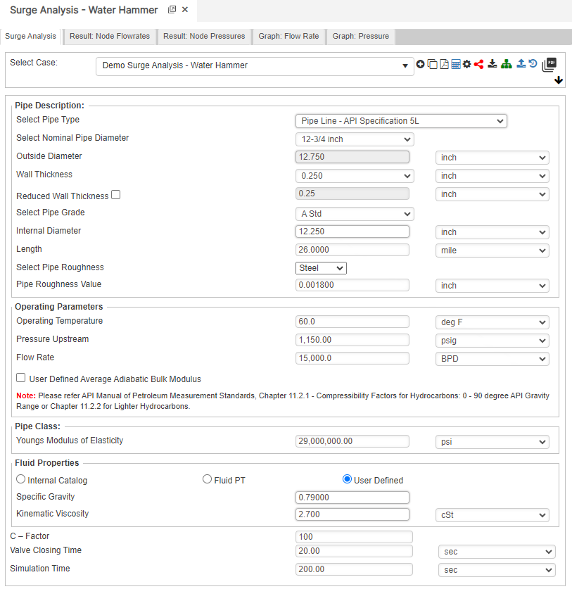
Input Parameters

• Flowing Temperature(°F)
• Liquid Specific Gravity
• Upstream Pressure(psig)
• Flow Rate(Barrels per Day)
• Internal Pipe Diameter(in)
• Kinematic Viscosity
• Length of Pipeline(mi)
• Upstream Elevation(ft)
• Downstream Elevation(ft)

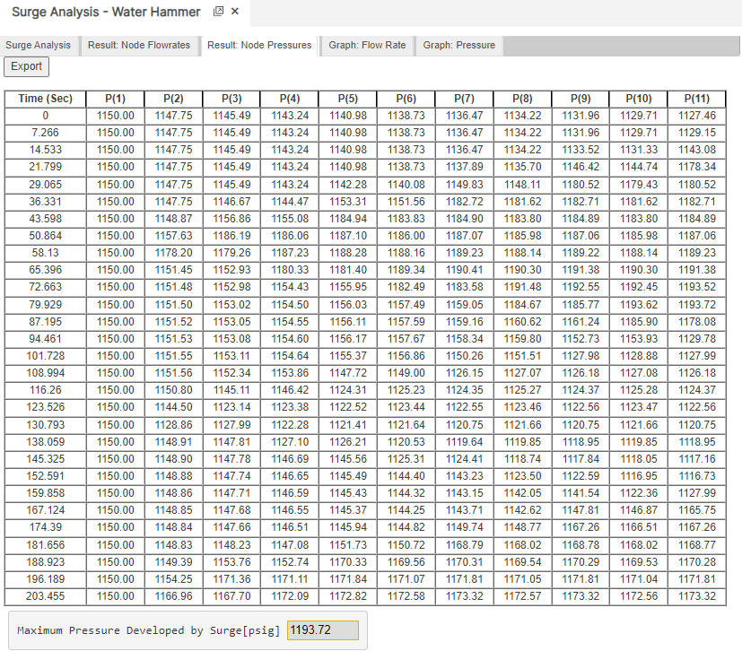
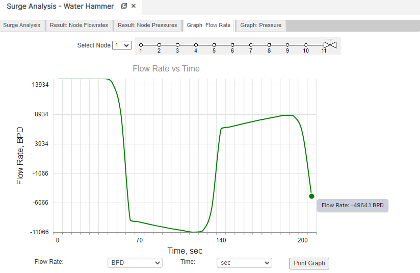
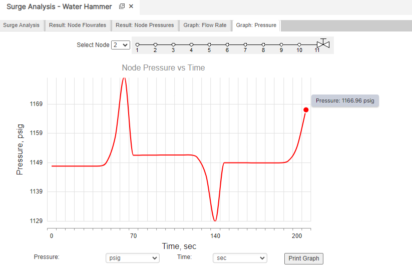
Surge Analysis – Water Hammer

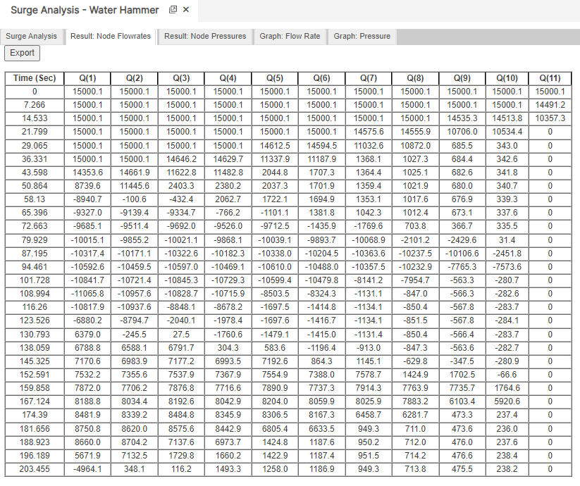
Part 2: Outputs/Reports

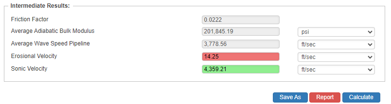
Results

• Friction Factor
• Average Adiabatic Bulk Modulus(psi)
• Average Wave Speed Pipeline(ft/sec.)
• Erosional Velocity (ft/sec.)
• Sonic Velocity (ft/sec.)

Surge Analysis – Water Hammer

References

• “Pipeline Rules of Thumb” Gulf Professional Publishing, Seventh Edition, McAllister, E. W.
• “Gas Pipeline Hydraulics”, Systek Technologies, Inc., Menon, Shahi E.
• “Advanced Pipeline Design”, Carroll, Landon and Hudkins, Weston R.
• American Gas Association (AGA), “Reference: Eq-17-18, Section 17, GPSA”, Engineering Data Book, Eleventh Edition
• Hydraulic Transients, McGraw-Hill, New York., Streeter, V.L. and Wylie, E.B. (1967)
• Water Hammer Analysis. Jour. Hyd. Div., ASCE., Vol. 88, HY3, pp79-113 May, Streeter, V.L. (1969)
• Unsteady flow calculations by numerical methods’, Jour. Basic Eng., ASME., 94, pp457-466, June. Streeter, V.L. (1972),
• Hydraulic Pipelines, John Wiley & Sons, J. P Tullis (1989)

FAQ