Objective

The user guide for the AC Mitigation PowerTool’s Steady State module serves to guide the user through modeling and mitigating AC corrosion under steady state conditions. This guide will cover creating and importing pipeline data, through modeling the effects of AC current on the pipeline, along with inputting and modeling the effects of mitigation on the pipeline.

Note: For further information related to the theory behind AC interference and mitigation, please refer to the AC Mitigation PowerTool Theory Guide. Certain terms in the AC Mitigation PowerTool (ACPT) User Guide are hyperlinked to corresponding sections of the Theory Guide for ease of access. Some of these terms may also be expanded upon in multiple sections of the Theory Guide. 

To view the field data required for operation of the AC Mitigation PowerTool, refer to Appendix C of the ACPT Theory Guide.

Importing Entities into ArcGIS

The first step to using the AC Mitigation PowerTool is to import pipeline and power line data into ArcGIS, creating entities representative of pipelines and power lines. This will allow the user to visualize the imported pipeline data and to create entities that can be edited and divided into sections. If users have the Navigator Addon licensed, this process will also add the entities into the Hierarchy Panel.

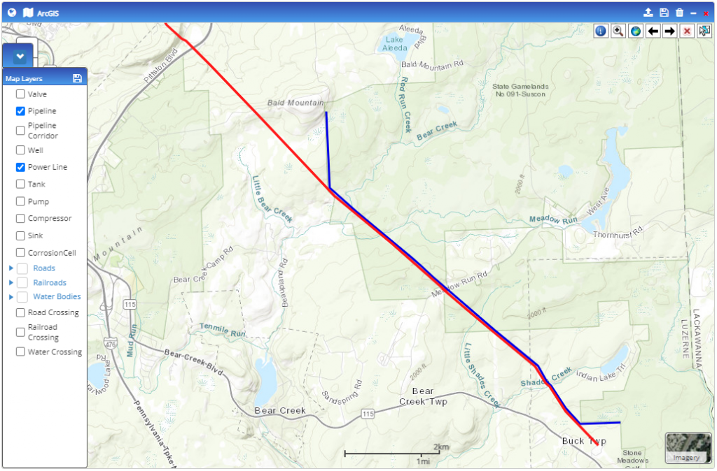
• Access the ArcGIS map by selecting ESRI Map from the blue ribbon at the top of the screen.
• Select the button in the lower left corner of the map, and check the boxes next to the entities that you would like to view. For the AC Mitigation PowerTool, Pipeline and Power Line are the most applicable entities.
• To import entities, in this case Power Lines and Pipelines, into the ArcGIS map:
  • Click on the button at the top right of the map to import pipeline and power line data.
  • Select either the Overwrite or Retain option, and then click Upload File (KML/Shape Files/GDB).
  • Select the applicable file and click Open.
  • In the dropdown of the entity that matches the imported file, select doc and click the adjacent Map Columns button.
  • Select the applicable fields from the dropdowns to their corresponding columns. Some fields will auto-populate. When all applicable fields are mapped, click Done.
  • Click Save Mapping
  • Click the button in the top right of the ArcGIS window to Save.
  • Repeat these steps for all entities that need to be imported, saving between each one.

Bringing the Imported Entities into the AC Mitigation PowerTool

Now that pipeline and power line data has been imported into ArcGIS, it is time to open the AC Mitigation PowerTool’s Steady State module and to bring in the power line and pipeline entities and data.

• Open the AC Mitigation PowerTool by hovering the Corrosion Tools dropdown on the top ribbon, then selecting AC Mitigation – Steady State, and lastly clicking AC Mitigation PowerTool GIS.
• Create a New Case
  • Users can manually input Latitude/Longitude or click the Lat/Long pin and click on the location in the ArcGIS map.
• Save the Case before proceeding.

Power Lines

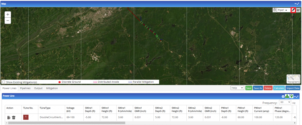
• To bring power lines into the ACPT, click on the power line in the ArcGIS Map to select it, and then click on the pin button outlined in red below to bring it into the Power Lines table. If users have access to the Navigator Addon, pipelines and powerlines can be imported by selecting the entity from the Hierarchy, and clicking the Hierarchy button adjacent to the pin button.

• Attributes of the power line will be carried over from the initially imported power line file, but users should click on the button in the Action box to verify and edit any applicable information about the power line and click Continue when finished. This step should be repeated for each power line individually. Click on the Save button in the top right after all power lines have been brought in.
• Power lines can also be manually added by clicking on the button, and all fields can be filled in by the user. Note that changing the Power Line Type will affect the number of Phase Wires and the Lat, Long field contains a default value that should be modified. 
• Be sure to specify the Frequency (Hz) in the top right of the Power Line table.
• The R (ohm/mile) field in the power line attribute editor denotes resistivity.
• Power Lines can be removed from the table by clicking the button in the associated Action box.
• SWire denotes Shield Wire, PWire denotes Phase Wire.
• GMR refers to the Geometrical Mean Radius of the associated wire, basically meaning the geometric mean of distances between the strands of a conductor.

Pipelines

• The same steps can be repeated in the Pipelines tab to bring Pipelines into the ACPT.
• To create Sections, users can either Add/Insert sections and edit them individually, Import Sections by downloading the template found through the Import Sections button and importing the filled-in template, or they can draw sections on the ACPT Map.
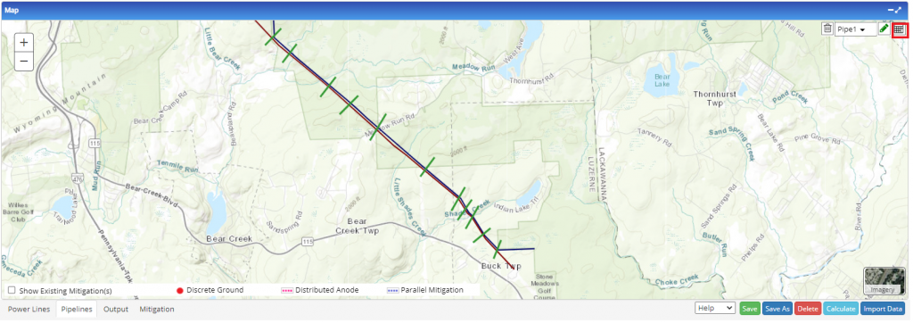
  •  The Draw Sections button (outlined in red in the image below) can be found in the upper right-hand corner of the ACPT map. Once the user has activated the Draw button, click once where the user would like to start the section line, and then double click where the user would like to end the section line. Sections can be based on topographical changes, cathodic protection factors, geometric changes, or any other factor decided upon by the user.
  • To delete extraneous section lines, simply right click the section line and click Delete.

• The Import Sections feature is also an effective way of incorporating Barnes Layer and soil resistivity data.
• Ensure that the correct line is selected as the Reference line in the dropdown at the top right of the map. 
• Click on the Calculate Angles and Distances (outlined in red in the image below) to populate the Sections and Pipe Section Depth Profile tables.
• Click the Save Button to ensure no work is lost
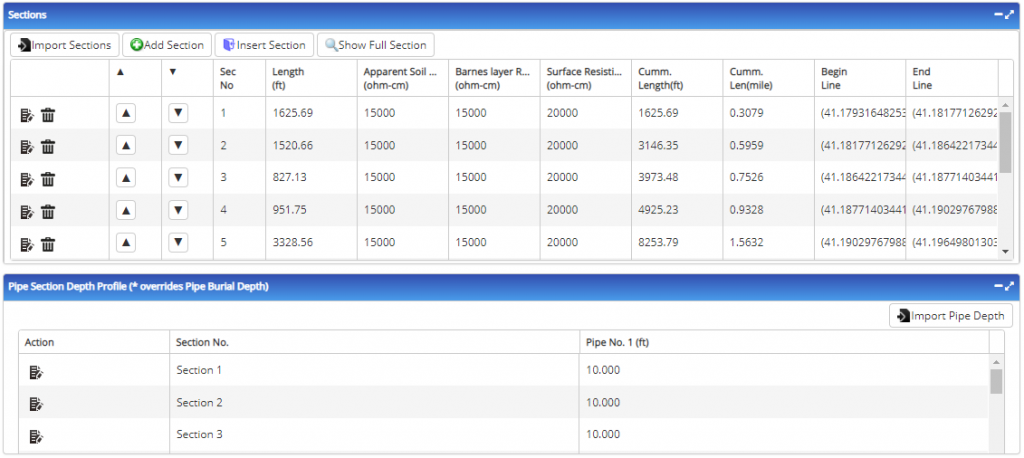
• Once the Sections have been generated, users can click on the buttons to edit any of the fields present in the Sections and Pipe Section Depth Profile tables. They can also click the button to delete sections that they wish to remove. Users can identify how sections on the Map correspond to sections in the Section table by hovering their cursors on the section on the map, reading the Section Number that appears, and referencing the Sec No column in the Sections Table. Once users have edited or deleted a Section in the Sections table, they can update the map to reflect these changes by clicking Save.
• The AC Mitigation PowerTool Theory Guide can provide more detail related to Pipeline Coating and AC interference.
• It is recommended to Save the Case and Map before proceeding.
• Note that the Pipe Section Depth Profile table can be edited, or Pipe Section Depth data can be imported using the Import Pipe Depth button, to incorporate depth of cover. This will override the Pipe Burial Depth values.

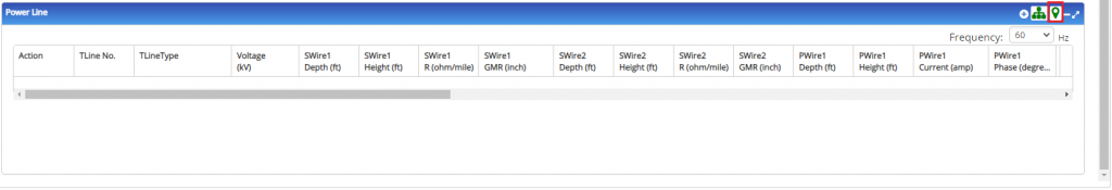
Output

• To populate the Output tab once the Pipeline sections have been generated, click on the Calculate button in the bottom right of the map.
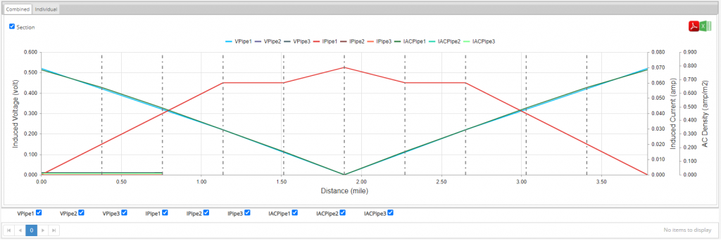
• In the Output section, users can view the induced voltages (blue line, labelled VPipe), induced current (red line, labeled IPipe), and AC current density (green line, labeled IACPipe) on the pipelines  either on individual graphs or combined into one graph.
• Users can also toggle the Section designations on or off by selecting or de-selecting the check box next to Section.
• Additionally, users get Quick View versions of the Sections, Results, Mitigation, Bond Connections, and Pipe Length Depth in this tab.
• Users can also download the case/report as an excel document or a PDF by clicking the buttons in the upper right corner of the Outputs tab.
• This AC Corrosion Rate table can provide guidance related to the likelihood of AC corrosion based on current density. More information can be found throughout the Theory Guide.

Mitigation

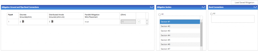
• In the Mitigation section, users can input Discrete Grounds, Distributed Anode Grounds, and Parallel Mitigation Wire Placement as forms of mitigation. The attributes of these can be edited by clicking on the button. Note that the Mitigation Ground and Pipe Bond Connections table is related to individual sections that are represented in the Mitigation Section column. Users can do each section individually, click the All checkbox to input mitigation for all sections at once, or select multiple sections by holding the Shift key and clicking the desired sections.
• When working with multiple pipelines, boxes can be checked in the Bond Connections section to indicate whether or not two pipes are bonded together.
• The (Ohm) box can be edited to indicate the resistance of the parallel mitigation wire.
• The Load Saved Mitigation button restores the previous mitigation settings in the event that users are experimenting with different permutations of mitigation and wish to quickly revert to the previous settings.
• Checking the “Show Existing Mitigation(s)” checkbox on the Map will display the input mitigation based on the legend at the bottom of the map. 
• Once the desired mitigation attributes have been input, clicking Calculate will return the user to the Output tab, where users can see the effects of the mitigation on the graphs.

Related Links