Hydraulics - Liquid

Introduction

The Pipeline Toolbox is home to many tools and calculators. The PLTB User’s Guide presents information, guidelines, and procedures for use during design and operations tasks for field or office applications.

Pipeline Hydraulic Fundamentals

For Fluids flowing in a pipeline between two points (A and B), the energy balance is subject to the following equation known as Bernoulli’s equation 2:

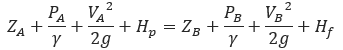
Where

𝑍_𝐴 = Elevation at point A

𝑍_𝐵 = Elevation at point B

𝑃_𝐴 = Pressure at point A

𝑃_𝐵 = Pressure at point B

𝑉_𝐴 = Velocity at point A

𝑉_𝐵 = Velocity at point B

𝑔 = gravity constant

𝛾 = gravity times the density of the fluid

𝐻_𝑝 = the equivalent head added to the fluid by a compressor at point A

𝐻_𝑓 = the total frictional pressure loss between points A and B

Several equations are available that relate the liquid flow rate with fluid properties, pipe diameter and length, and upstream and downstream pressures. These equations are listed as follows:

1. Darcy-Weisbach
2. Colebrook – White
3. Hazen-Williams
4. Heltzel
5. A.R. Aude
6. Shell/MIT

In addition, two other equations are primarily used for calculating pressure drops and flow rates.

1. Darcy-Weisbach Pressure Drop per Mile
2. Surge Analysis – Water Hammer

We will discuss each of these equations, their limitations, and their applicability.

Erosional and Sonic Velocity has been added to the following Modules and Calculations.

1. Colebrook – White
2. Darcy – Weisbach
3. Darcy – Weisbach Pressure Drop per Mile
4. Surge Analysis – Water Hammer

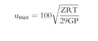
Erosional Velocity

Pipe erosion begins when velocity exceeds the value of C/SQRT(ρ) in ft/sec, where ρ = gas density (in lb./ft3) and C = empirical constant (in lb/s/ft2) (starting erosional velocity). We used C=100 as API RP 14E (1984).  However, this value can be changed based on the internal conditions of the pipeline.  The following equation is used for the calculation.

Inputs

• C – Factor (dimensionless)
• Compressibility Factor (dimensionless)
• Gas Gravity (dimensionless)
• Operating Pressure (psig)
• Operating Temperature (deg F)

Sonic Velocity

The maximum possible velocity of compressible fluid gas/liquids in pipe is called sonic velocity.

Inputs

• K = Cp/Cv – the ratio of specific heats at constant pressure to constant volume (fluid directive)
• G=32.2 ft/sec
• R=1544/mol. Wt.
• T = Absolute temperature in deg R

K = A + B(P) – C(T)^1/2 – D(API) – E(API) – E(API)² + F(T)(API)

Sonic Velocity is in ft/sec.

Module/Application

• Darcy – Weisbach
• Colebrook – White
• Hazen – Williams
• Heltzel
• A.R. Aude
• Shell/MIT
• Darcy – Weisbach Pressure Drop Per Mile
• Surge Analysis – Water Hammer

References

• “Pipeline Rules of Thumb” Gulf Professional Publishing, Seventh Edition, McAllister, E. W.

• “Gas Pipeline Hydraulics”, Systek Technologies, Inc., Menon, Shahi E.

• “Advanced Pipeline Design”, Carroll, Landon and Hudkins, Weston R.

• American Gas Association (AGA), “Reference: Eq-17-18, Section 17, GPSA”, Engineering Data Book, Eleventh Edition

• Hydraulic Transients, McGraw-Hill, New York., Streeter, V.L. and Wylie, E.B. (1967)

• Water Hammer Analysis. Jour. Hyd. Div., ASCE., Vol. 88, HY3, pp79-113 May, Streeter, V.L. (1969)

• Unsteady flow calculations by numerical methods’, Jour. Basic Eng., ASME., 94, pp457-466, June. Streeter, V.L. (1972),

• Hydraulic Pipelines, John Wiley & Sons, J. P Tullis (1989)

Appendix of Definitions

Colebrook-White – The Colebrook-White equation is recommended for use by those unfamiliar with pipeline flow equations since it will produce the greatest consistency of accuracy over the widest possible range of variables.

Darcy-Weisbach – Darcy-Weisbach equations are valid for steady-state flow. The friction factor – λ -depends on the flow, (laminar, transient, turbulent, Reynolds number) and the internal roughness of the pipe.  The friction coefficient can be calculated by the Colebrook-White equation.

Hazen – Williams – Used for primarily water lines associated with production facilities.  Limited to Reynolds numbers in the range of Re = 4,000 to 1,000000.

Heltzel – One of the oldest equations is which is still being used for Reynolds values in the range of Re = 4,000 to 57,600.

T.R. Aude – This equation is accurate for Reynolds numbers in a range of Re:

– 6,000 to 130,000 for 8″ and 12″ crude oil lines.

– over 57,000 for 6″ and 8″ refined product lines.

Shell/MIT – These equations are primarily used for calculating pressure drops and flow rates.  However, a modified Reynolds number must be used.

Related Links