Wheel Load Analysis

Introduction

Wheel Load Analysis was designed to calculate the overburden and vehicle loads on buried pipe with a Single Layer System (soil only) or a Double Layer Systems (timbers, pavement and soil). The information used to design this program was taken from the Battelle Petroleum Technology Report on “Evaluation of Buried Pipe Encroachments” which considered the theoretical work done by M.G. Spangler on overburden and vehicle loads on buried pipe. This analysis does not evaluate cyclic loading, but the API 1102 calculation does.

Variables and Boundary Conditions

1. Depth of Carrier Pipe

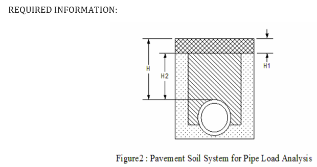
• The depth of the carrier pipe, H, is measured from the top of pavement, rig mats, or soil (if neither pavement nor rig mats exist) to the pipeline crown.
  • is used to establish the impact factor, F_i used in the design methodology.
  • is calculated by H = H₁ + H₂
• H₁ – Thickness of the pavement layer, if there is a pavement layer
  • Rig mats are considered a part of the pavement layer
  • Has units of inches (in)
  • (see Figure 2)
• H₂ – vertical depth from the ground to the top of the pipe
  • If there is a surface layer of pavement or rig mats, this measurement begins at the bottom of that pavement layer
  • Has units of feet (ft)

Trench Width

• Width of the trench, B, that was excavated during construction
• Has units of feet

Weight per unit Volume of Backfill

• Weight per unit Volume, D_s
• Has units of pounds per cubic foot (lb/ft³)

DIAMETER.

• The diameter, D, is the outside pipe diameter
• has units of inches.
• The range of D is 2.000 to 42.000 in.
• The default value is D = 12.750 in.

WALL THICKNESS.

• The pipe wall thickness, T, has units of inches.
• The wall thickness to diameter ratios must be within the range of wt./D = 0.01 to 0.08.

Concentrated Surface Load

• The concentrated surface load, L_w, is the force applied by the wheel to the ground, vs. the gross weight weight
• Has units of pounds (lbs)
• see Section 4,Page 11

SPECIFIED MINIMUM YIELD STRENGTH.

• The specified minimum yield strength, SMYS,
• Has units of pounds per square inch (psi)
• has a range of allowable values covering steel grades A25 (SMYS = 25000 psi) to X-80 (SMYS = 80000 psi).
• The SMYS is also used to establish the girth and longitudinal weld fatigue endurance limits.

P – Pipe Internal Pressure (psi.)

2. Design Class

• Design Class of the pipeline being analyzed is defined by §192.5 Class Locations
• The allowable range is from 1 to 4
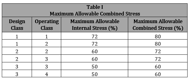
• Is used to find the Maximum Allowable Combined Stress (% SMYS), see Table I.
• Table I: Maximum Allowable Combined Stress

• Design Class	Operating Class	Maximum Allowable Internal Stress (%)	Maximum Allowable Combined Stress (%)
  1	1	72	80
  1	2	72	80
  2	2	60	72
  2	3	60	72
  3	3	50	60
  3	4	50	60

3. Soil Type

• Which is used to find the friction force coefficients (Km)
• Table 2:
  

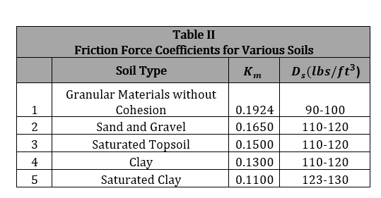
  	Soil Type	Friction Force Coefficient
  1	Granular Materials without Cohesion	0.1924	90-100
  2	Sand and Gravel	0.1650	110-120
  3	Saturated Top Soil	0.1500	110-120
  4	Clay	0.1300	110-120
  5	Saturated Clay	0.1100	123-130

  • The soil types and coefficients given in this table represent the range that could normally be expected.
    • Saturated clay has little internal friction so that it has the smallest value for Kμ. This implies that almost all of the soil load is carried by the pipe.
    • Granular materials have a great deal more internal friction. Their value of Kμ is higher which leads us to the conclusion that the pipe carries less of the backfill load.
    • Marsh and bog areas, however, have friction properties more similar to saturated clay such that a value for Km equal to 0.110 should be used in these areas.
  • Spangler, in his work, recommends using the value for clay in most instances.
    • Higher values may be used when there is adequate evidence that the internal friction is higher and warrants a higher value of Kμ.
    • Spangler’s recommendation provides a conservative estimate for common buried pipe situations.
• W_c=(1-e^((-2K_μ (H_2⁄B)) ))/2Kμ D_s B^2 (83.3×10^(-3))

4. Pavement Type

• Is used to find the elastic constants for layered media analysis (E1, E2, G1, & G2) see Table III & Figure 2.
• A Pavement Type must be determined in order to select an Impact Factor (I) to be used in the Wv equation.
  • Table III: Impact Factor and Elastic Constants for Layered Media Analysis
    

    Pavement Type	Impact Factor -I	Elastic Constant -E (psi)	Poisson’s Ratio – G
    No Pavement	1.5	1.5×104	0.35
    Asphalt	1.3	1.0×105	0.40
    Timber Mats (2’x12″ min.)	1.2	1.2×106	0.25
    Concrete	1.0	2.0×106	0.15

• The variables E1 & G1 will be used to represent the elastic constants for the top layer and E2 & G2 will be used to represent the elastic constants for the soil.
  • See Figure 2 for a visual explanation of the elastic constants for the top layer and the soil.
  • These values will also be used in the Wv equation.

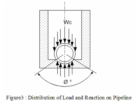
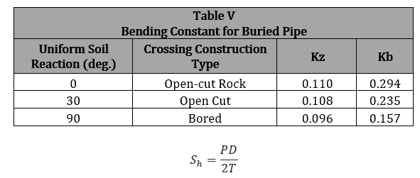
5. The Pipeline Construction Type which is used to find the bedding constants for buried pipe (Kb & Kz), see Table V & Figure 3.

REQUIRED INFORMATION IF LONGITUDINAL BENDING STRESS OCCURS:

6. All the above information along with values for the following variables:
X – Longitudinal Distance over which Deflection occurs (ft.)
Y – Vertical Deflection (in.)

Workflow

As a first estimate of the soil load on the pipe it could be assumed that the backfill soil slides down the 0trench walls without friction. Additionally, assume that all soil above the pipe is supported by the pipe itself and that the backfill soil on either side of the pipe does not assist in this support.

These assumptions are very conservative, but they help a great deal in initial understanding of the method of solution. The assumptions yield a soil load on the pipe equal to the weight of the backfill soil above the pipe. This analysis provides an estimate of soil loads on the buried pipe if nothing else is known about the system.

The basic analysis developed by M.G. Spangler follows similar arguments to that given above. In this analysis, Spangler includes frictional forces between the trench wall and the backfill. This permits the weight of the overburden to be partially carried by the surrounding soil and reduces the total soil load on the pipe. The resulting equations for calculating the pipe load due to overburden are as follows:

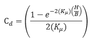
𝐶_𝑑 − Trench Coefficient

B − Trench Width (ft)

𝐻 − H₁ +H₂ , Pipe Depth (ft)

𝐾_𝜇 − Coefficient of friction force between the backfill soil and the trench wall.

Cd determines how much load is carried by the pipe. If there is no soil friction Cd becomes equal to H/B and the entire backfill load must be supported by the pipeline. The term Km provides a coefficient of friction force between the backfill soil and the trench wall. A high value of Km implies that friction between the backfill and trench wall is high and the weight of the backfill is supported largely by the wall friction. A low value implies that there is little friction encountered and the backfill is allowed to settle more such that the weight must be supported by the pipe. Table II provides values of Km used in the program for five different soil types. Also, in Table II are examples of values for Ds, the
density which is the weight per unit of backfill, which may be used if an actual value is not known. Note: If a value for Ds is already given use that value instead of the one in Table II.

The soil types and coefficients given in this table represent the range that could normally be expected. Saturated clay has little internal friction so that it has the smallest value for Kμ. This implies that almost all of the soil load is carried by the pipe. Granular materials have a great deal more internal friction. Their value of Kμ is higher which leads us to the conclusion that the pipe carries less of the backfill load. Spangler, in his work, recommends using the value for clay in most instances. Higher values may be used when there is adequate evidence that the internal friction is higher and warrants a higher value of Kμ. Spangler’s recommendation provides a conservative estimate for common buried pipe situations. Marsh and bog areas, however, have friction properties more similar to saturated clay such that a value for Km equal to 0.110 should be used in these areas.

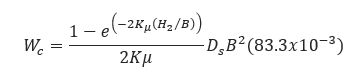
𝑊_𝑐 − Load per unit Length of the Pipe due to Overburden(lbs/in)

𝐵 − Trench Width(ft)

𝐻₂ − Cover, Vertical Depth from the Ground Surface to Top of Pipe(ft)

𝐷_𝑠 − Density which is the Weight per unit of Backfill(lbs/ft³)

𝐾_m − Coefficient of Friction Force between the Backfill Soil and the Trench Wall.

A Pavement Type must be determined in order to select an Impact Factor (I) to be used in the Wv equation. Table III provides Impact Factor values for the three different pavement types used in this program. A Pavement Type is also used to select the elastic constants for layered media analysis. The variables E1 & G1 will be used to represent the elastic constants for the top layer and E2 & G2 will be used to represent the elastic constants for the soil. See Figure 2 for a visual explanation of the elastic constants for the top layer and the soil. These values will also be used in the Wv equation. Table IV provides the values for the three different pavement materials used in this program.

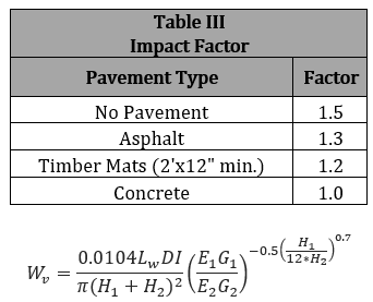
𝑊_𝑣 − Average Load per unit Length of the Pipe for Vehicular Load(lbs/in)

𝐷 − Outside Diameter of the Pipe(in)

𝐸₁ − Modulus of Elasticity of the Top (timber or pavement)Layer(lbs/in²)

𝐸₂ − Modulus of Elasticity of the Soil Cover(lbs/in²)

𝐺₁− Poisson′s Ratio of the Top (timber or pavement) Layer

𝐺₂ − Poisson′s Ratio of Soil Cover

𝐷_𝑠 − Density which is the Weight per unit of Backfill(lbs/ft³)

𝐻₁ − Thickness of the Pavement Layer (“0” is used when there is no pavement) (in.)

𝐻₂ − Cover, Vertical Depth from the Ground Surface to Top of Pipe(ft)

𝐷_𝑠 − Density which is the Weight per unit of Backfill(lbs/ft³)

𝐼 − Impact Factor

𝐿_𝑤−Concentrated Surface Load (16000 lbs is recommended when the max. is unknown)(lbs)

Examination of equation Wv shows that this equation also may be used with a Single Layer System because the Pavement Material on the Top Layer chosen is “Soil”, which makes E1 equal to E2, G1 equal to G2, and H1 equal to zero which cancels out the second and third part of the equation. Thus, when there is no pavement layer the revised equation will provide a solution for soil cover only. Table IV provides the values for E1, E2, G1 & G2 that will be used in the program.

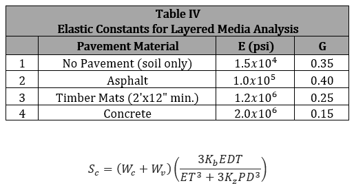
𝑆_𝑐 − Circumferential Stress due to Pipe Wall Deflection(psi)

𝐷 − Outside Diameter of the Pipe(in)

𝐸 − Pipe Material Modulus of Elasticity (2.9 x 10⁷)

𝐾_𝑏 − Bending Coefficient which is a function of the crossing construction types

𝐾_𝑧 − Deflection Coefficient which is a function of the crossing construction types

𝑃 − Pipe Internal Pressure (psi)

𝑇 − Pipe Wall Thickness(in)

𝑊_𝑐 − Load per unit Length of Pipe due to Overburden(lbs/in)

𝑊_𝑣 − Average Load per unit Length of Pipe for Vehicular Load (lbs/in)

Note that the equation Sc includes pressure in the denominator so that bending stresses are reduced by increasing pressure.

Equation Sc, as well as equation St, have two constants which depend upon the bedding material upon which the pipe is placed. This bedding material is based on the crossing construction type. When the pipe is placed on a rigid bedding such as an Open Cut-Rock, little soil deformation occurs so that the load application area on the bottom is very small.
However, if the pipe is placed on soil, the support conforms to the pipe somewhat and the load is distributed over a larger area (See Figure 3). The latter case produces less pipe stress and is preferable. Spangler’s formulation includes both of these possibilities in order to provide a conservative estimate for the rigid bedding case without penalizing the soil bedding case. It does so by varying the constants Kb and Kz. Spangler’s recommended values for the constants are provided in Table V.

𝑆_ℎ − Hoop Stress due to Internal Pressure(psi)

𝐷 − Outside Diameter of the Pipe(in)

𝑃 − Pipe Internal Pressure(psi)

𝑇 − Pipe Wall Thickness(in)

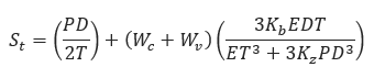
St is the total circumferential stress in the pipe wall due to pressure (hoop) stress and bending stresses resulting from circumferential flexure caused by external loads measured in PSI. The first term on the right-hand side of the equation is the formula for hoop stress due to internal pressure (Sh) and the second term is the formula for circumferential stress due to pipe wall deflection (Sc). Longitudinal Bending Stress (Sb) is when the overburden and vehicle load on buried pipelines will cause pipe settlement into the soil in the bottom of the trench. This settlement occurs because soil is not as stiff as the pipe and will deform easily as the pipe is “pushed” downward. Under uniform soil conditions and overburden loading, the pipe will settle evenly into the trench bottom along its entire length. Soil is not generally uniform, however, and regions of “softer” soil will occur adjacent to regions of stiff soil, so that the pipe will settle unevenly and hence bending will occur. A load that is applied on only one portion of a pipeline will cause the section of pipe under the load to settle more than the unloaded pipe, such that bending will also result. Longitudinal bending stress occurs in tension on the outside of the bend and in compression on the inside of the bend. Tensile stress is represented with a positive value for Sb; conversely, compressive stress takes a negative value for Sb. The longitudinal bending stress is calculated as follows:

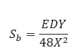
𝑆_𝑏 − Longitudinal Bending Stress(psi)

𝐷 − Outside Diameter of the Pipe(in)

𝐸 − Pipe Material Modulus of Elasticity(2.9 x 10⁷)

𝑋 − Longitudinal Distance over which Deflection occurs(ft)

𝑌 − Vertical Deflection(in)

A negative value will be used when calculating the total combined stress (S). This will result in a larger (more conservative) combined stress. Note: If longitudinal bending stress does occur, click onto the designated box next to “Longitudinal Bending Stress”. If the box is not marked, then the program will assume “0” for Sb.

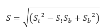
𝑆 − Total Combined Stress by Von Mises(psi)

𝑆_𝑏 − Longitudinal Bending Stress(psi)

𝑆_𝑡 − Total Circumferential Flexure caused by External Loads(psi)

Note that if longitudinal bending stress is not present then the S will equal St. The final calculation is % SMYS. This is calculated to determine if the current conditions exceed the Maximum Allowable Combined Stress determined by Transcontinental Gas Pipe Line Corporation.

S – Total Combined Stress by Von Mises(psi)
SMYS – Specified Minimum Yield Strength(psi)

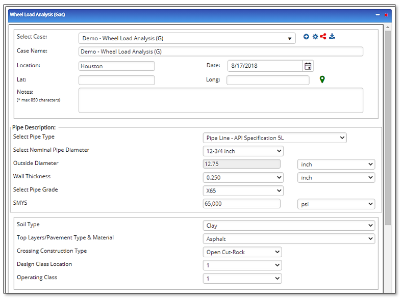
Input Parameters

1. To create a new case, click the “Add Case” button
2. Select the Wheel Load Analysis application from the Pipeline Crossing module.
3. Enter Case Name, Location, Date and any necessary notes.
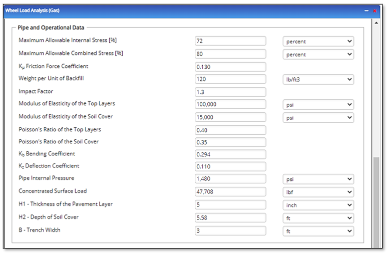
4. Fill out all required fields.
5. Make sure the values you are inputting are in the correct units.
6. Click the CALCULATE button.

• Potential Nominal Pipe Size(in):(1/8” – 48”)
• Pipe Outside Diameter(in):(0.625” – 48”)
• Pipe Wall Thickness(in):(0.068”- >2”)
• Design Location
• Operation Class
• Soil Type
• Top Layer/Pavement Type and Material
• Crossing Construction Type
• Maximum Allowable Internal Stress
• Maximum Allowable Combined Stress
• Friction Force Coefficient
• Weight Per Unit of Backfill
• Impact Factor
• Modulus of Elasticity of the Top Layer
• Modulus of Elasticity of the Soil Cover
• Poisson’s Ratio of the Top Cover
• Poisson’s Ratio of the Soil Cover
• Bending Coefficient
• Deflection Coefficient
• Pipe Internal Pressure
• Concentrated Surface Load
• Vertical Depth of the Soil Cover
• Thickness of the Pavement Layer
• Trench Width
• Specified Minimum Yield Stress:(24000psi-80000psi)
• Pipeline Length

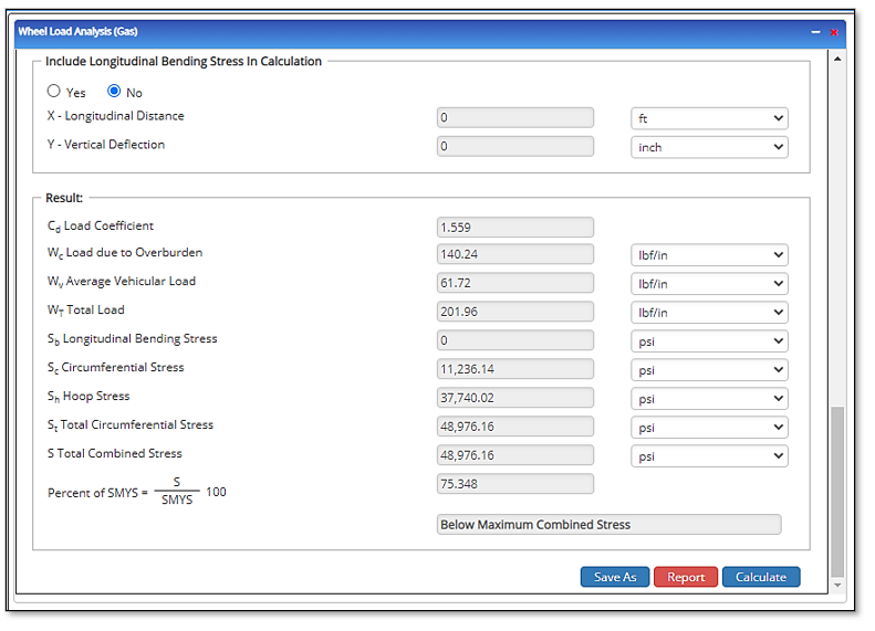
Outputs/Reports

1. View the results.
2. If an input parameter needs to be edited be sure to hit the CALCULATE button after the change.
3. To SAVE, fill out all required case details then click the SAVE button.
4. To rename an existing file, click the SAVE As button. Provide all case info then click SAVE.
5. To generate a REPORT, click the REPORT button.
6. The user may export the Case/Report by clicking the Export to Excel/PowerPoint icon.
7. To delete a case, click the DELETE icon near the top of the widget.

• Load Coefficient
• Load due to Overburden
• Average Vehicular Load
• Total Load
• Longitudinal Bending Stress
• Circumferential Stress
• Hoop Stress
• Total Circumferential Stress
• Total Combined Stress
• Percent Of SMYS
• Status

Tutorial Videos

• Finding Road Crossings (2 min 52 sec)
• Crossings Workflow Demo (4 min 50 sec)