PLTB Gas Services Hydraulics – Gas

Introduction – Hydraulics

The Pipeline Toolbox is home to many tools and calculators. The PLTB User’s Guide presents information, guidelines, and procedures for use during design and operations tasks for field or office applications.

Pipeline Hydraulic Fundamentals

For Fluids flowing in a pipeline between two points (A and B), the energy balance is subject to the following equation known as Bernoulli’s equation 2:

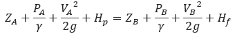
Where

𝑍_𝐴 = Elevation at point A
𝑍_𝐵 = Elevation at point B
𝑃_𝐴 = Pressure at point A
𝑃_𝐵 = Pressure at point B
𝑉_𝐴 = Velocity at point A
𝑉_𝐵 = Velocity at point B
𝑔 = gravity constant
𝛾 = gravity times the density of the fluid
𝐻_𝑝 = the equivalent head added to the fluid by a compressor at point A
𝐻_𝑓 = the total frictional pressure loss between points A and B

According to the results of an in-depth analysis, the industrial equations can produce large amounts of error when compared to a process simulator analysis with the same pipe specifications and conditions. The following table shows the results of the equation study:

Table 1: Conventional Hydraulic Equation Analysis

Equation Name	Range of Error
Panhandle	3.5-10%
Colebrook	2.4-10%
Modified-Colebrook	1.0-8.8%
AGA	0.2-15%
Weymouth	39-59%
IGT	7.6-17%
Spitzglass	88-147%
Mueller	13-20%

The error produced by these equations is due to the assumptions used to derive the equation from the General Flow Equation. Also, extremely large amounts of error occurred when the equations were applied outside their intended pipeline environment. This error could directly affect theoretical optimal pipeline diameter and cause it to be significantly different from the actual optimal pipe diameter.

We will discuss each of these equations, their limitations, and their applicability.

Erosional and Sonic Velocity has been added to the following Modules and Calculations.

Erosional Velocity

Pipe erosion begins when velocity exceeds the value of C/SQRT(ρ) in ft/s, where ρ = gas density (in lb./ft3) and C = empirical constant (in lb./s/ft2) (starting erosional velocity). We used C=100 as API RP 14E (1984). However, this value can be changed based on the internal conditions of the pipeline. The following equation is used for the calculation.

Inputs

C – Factor (dimensionless)
Compressibility Factor (dimensionless)
Gas Gravity (dimensionless)
Operating Pressure (psig)
Operating Temperature (deg F)
PLTB

Erosional Velocity is in ft/sec

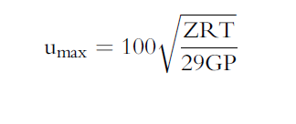
Sonic Velocity

The maximum possible velocity of compressible fluid gas/liquids in pipe is called sonic velocity.

Inputs

K = Cp/Cv – the ratio of specific heats at constant pressure to constant volume (fluid directive)
G=32.2 ft/sec
R=1544/mol. Wt.
T = Absolute temperature in deg R

K = A + B(P) – C(T)^1/2 – D(API)2 + F(T) (API)

Sonic Velocity is in ft/sec

Module/Application

Gas Correlations

Panhandle A
- Uses an empirical efficiency factor of 0.92 for partially turbulent flow conditions. It is suitable for Reynolds numbers from 5 x 106 to 11 x 106. Smaller diameter lines such as 12″ and below, the efficiency factors need to be reduced.
Panhandle B
Weymouth
A.G.A. Fully Turbulent Flow
Colebrook – White
FM – Fundamental Equation
IGT Distribution Equation
Mueller – High Pressure
Mueller – Low Pressure
Pittsburg
Spitzglass

Tutorial Videos

Leveraging a Defined Fluid in PLTB (60 sec)

References

McAllister, E. W., “Pipeline Rules of Thumb” Gulf Professional Publishing, Seventh Edition
Menon, Shahi E., “Gas Pipeline Hydraulics”, Systek Technologies, Inc.
Carroll, Landon and Hudkins, Weston R., “Advanced Pipeline Design”
American Gas Association (AGA), “Reference: Eq-17-18, Section 17, GPSA”, Engineering Data Book, Eleventh Edition