PRCI Thermal Analysis Model for Hot-Tap Welding 

Introduction

This User Guide describes the use of the PRCI Thermal Analysis Model for Hot-Tap Welding (also referred to as PRCI Hot Tap). The model is intended to provide welding engineers with guidance for establishing safe parameters for welding onto in-service pipelines (hot-tap welding).

There are two primary concerns with welding onto in-service pipelines. The first is for welder safety during welding, since there is a risk of the welding arc causing the pipe wall to be penetrated allowing the contents to escape. The second concern is for the integrity of the pipeline following welding, since welds made in-service cool at an accelerated rate as the result of the ability of the flowing contents to remove heat from the pipe wall. These welds, therefore, are likely to have hard heat-affected zones (HAZ) and a subsequent susceptibility to hydrogen cracking. The model allows burnthrough risk to be controlled by limiting inside surface temperature and hydrogen cracking risk to be controlled by limiting weld cooling rates.

The use of this model is not a substitute for procedure qualification. The model provides guidance for establishing safe parameters, but provides no means for demonstrating that these parameters are practical under field conditions. To demonstrate that the parameters are practical, a welding procedure based on these predictions should be qualified under simulated conditions. A brief history of cooling rate prediction methods for welds made onto in-service pipelines is given in Appendix A.

Overview

Entering Data

The initial steps to using the PRCI Hot Tap software consist of creating a New Case and selecting the appropriate Geometry and Pipe Contents. The user can select between Sleeve, Branch, Bead On Pipe, and Heat Sink Capacity for the Geometry, and can select between Gas and Liquid for Pipe Contents. The user should also select the appropriate Unit type (US or Metric) by clicking the button outlined in red in the image below. 

There are three data input panels: Pipe Joint, Weld Conditions, and Pipe Contents. Each panel contains a data integrity check routine. Clicking on the Check/Correct button (outlined in red in the image below) will check that the value for each parameter entered falls within pre-defined limits. These limits are shown in Table 1 below. If a given value falls outside of these limits, an error message will be displayed. Also, be sure to regularly Save using the button in the bottom right of the window.

Pipe Joint

The Pipe Joint data input panel contains field for entering details pertaining to the pipe material of interest and other details depending on which geometry has been selected. This input panel is shown in Figure 7 for a sleeve-fillet weld example. Illustrations of the three weld geometries are shown in the images below. Fields pertaining to the pipe material include Material, Outer Diameter, Thickness, Temperature, and Ambient Temperature. For cases involving a sleeve-fillet weld, fields pertaining to other details include Material, Thickness, Temperature, and Gap Between Pipe and Sleeve. For cases involving branch-groove welds, fields pertaining to other details include Material, Thickness, Temperature, Branch Root Gap, Angle Between Pipe and edge of Branch (i.e. the branch bevel angle), and Branch Outer Diameter. For Bead-on-Pipe or Heat-Sink Capacity cases, no other details are required.

The Pipe Joint data input panel also contains a Chemistry of Base Metal section used for Max Hardness Prediction. This section is only required if the user requires HAZ hardness predictions calculated using the Yurioka algorithm, the use of which is described later in this User Guide. If base metal chemistry is entered, hardness predictions will appear in tabular form on the printed report after running the finite element solver and as part of the enhanced heat input selection curves.

Weld or Heating Conditions

The second data input panel is Weld Conditions for Sleeve, Branch, and Bead-on-Pipe cases, or Heating Conditions for Heat-Sink Capacity cases.

The Weld Conditions data input panel contains fields for entering details pertaining to the welding parameters. This input panel, which allows multiple records to be run from a single case, is shown in the image below. After entering an optional weld description, options for entering welding parameters include Enter Weld Parameters of Enter Heat Input. Selecting Enter Weld Parameters allows specific values for welding current, voltage, and travel speed to be entered. Selecting Enter Heat Input requires that only a value for the resulting heat input is entered – the software selects specific values for welding current, voltage, and travel speed according to a preset algorithm. These specific values are shown as a function of heat input in the images below.

For cases where Enter Welding Parameters is selected, the fields pertaining to the welding parameters include Electrode Type, Electrode Diameter, Weld Speed, Arc Voltage, and Weld Current. For cases where Enter Heat input is selected, the fields pertaining to the welding parameters are the same except Heat Input replaces Weld Speed, Arc Voltage, and Weld Current.

A field for entering the arc efficiency of the welding process is also provided on the Weld Conditions data input panel. A pull-down menu containing arc efficiency for common welding processes is provided. A user-defined value for arc efficiency can also be entered.

The counter at the bottom of the Weld Conditions data input panel what Record is currently being displayed. To enter another Record, the user can click the New Record button, to delete a Record by clicking the Delete Record button, toggle between Records using the Next and Prev Record arrows, and toggle to the First and Last Records by using the First and Last buttons respectively.

The Heating Conditions data input panel for Heat-Sink Capacity cases is shown in the image below. This pane is similar to the Weld Conditions data input panel except it contains fields for entering data pertaining to torch heating conditions.

Pipe Contents

The Pipe Contents data input panel contains fields for entering details pertaining to the pipe contents. This input panel is shown in the image below for a gas pipeline contents example. Options for entering the flow rate include Linear Flow Rate or Volumetric Flow Rate. Fields pertaining to the Pipe Contents include Gas (or Liquid) Type, Linear (or Volumetric) Flow Rate, Temperature, and Pressure. For cases involving gas pipeline contents, a dropdown menu containing a list of common gases is provided. For cases involving liquid pipeline contents, a dropdown menu containing a list of common liquids is provided.

Generating the Results

After filling out all applicable fields in the Pipe Joint, Weld Conditions, and Pipe Contents tabs, users should be sure to Save their inputs using the Save Case button in the Case Header. After all inputs have saved, all inputs can be reviewed in PDF format using the Review Input button near the top of the widget. Next, users should click the Calculate button, resembling a calculator, in the case header. A popup window stating that the “Engine executed successfully” will indicate successful calculation of the results. Once the engine has been executed, users are able to click View Graph Results for Heat Input to Cooling Time graphs (view can be modified using the buttons at the top to specify which charts should be visible) and are able to generate a PDF report with the F.E.A. Result by clicking the Generate Report button in the case header.

If a PDF is not appearing in an additional tab after clicking either the Review Inputs or Generate Report buttons, users should try disabling their browser’s pop-up blocker, as this can interfere with the opening of additional tabs.

Using the Results

Controlling Burnthrough Risk

The inside surface temperature predictions are used to control the risk of burnthrough. Safe parameters are defined as those which produce an inside surface temperature of less than 1800°F (982°C) when using low-hydrogen electrodes or less than 1400°F (760°C) when using cellulosic-coated electrodes. In a series of previously conducted experiments, Battelle observed that burnthrough tended to occur when the inside surface temperature exceeded 2300°F (1260°C). The 500°F (278°C) temperature difference between this and the 1800°F (982°C) limit was introduced as a margin for safety. For individual cases that result in an inside surface temperature greater than the limits established by Battelle, an asterisk is provided adjacent to the inside surface temperature prediction on the printed report.

Controlling Hydrogen Cracking Risk

The weld cooling rate and cooling time between 800 and 500°C (△t_8-5) predictions are used to control the risk of hydrogen cracking. Hydrogen cracking susceptibility tends to increase with increasing hardness and hardness tends to increase with faster weld cooling rates (or shorter △t_8-5 times). There are two ways to use the results to control the risk of hydrogen cracking: the chemical composition method and the carbon equivalent method. The use of the latter is less precise but requires fewer details of the pipe material composition.

Chemical Composition Method

Knowing the predicted △t_8-5 time and the chemical composition of the pipe material, a previously developed algorithm, such as the one built into the software that was developed by Yurioka, can be used to predict the HAZ hardness. The hardness level above which hydrogen cracking can be expected to occur, or the critical hardness level, depends on the carbon equivalent level of the materials and on the hydrogen level of the welding process. The critical hardness level for in-service welds is shown as a function of carbon equivalent level and weld hydrogen level in Figure 20 below. This criteria, which is a modification of previous work by Matharu and Hart, was developed for welds made under simulated  in-service conditions during earlier work at EWI.

If base metal chemical composition is entered in the Pipe Joint data input panel, hardness predictions will appear in tabular form on the printed report after running the finite-element solver. The solver predicts HAZ hardness using the Yurioka algorithm and the predicted △t_8-5 time. To evaluate the risk of hydrogen cracking, the user can compare the predicted hardness to those shown in Figure 20 below. Alternatively, an enhanced heat input selection curve can be plotted from which the required heat input can be determined. 

To plot enhanced heat input selection curve, click on the View Graph Results button. An example of an enhanced heat input selection curve is shown below in Figure 22. The required heat input is determined by selecting the critical hardness for the carbon equivalent level and weld hydrogen level of interest from Figure 20, selecting the corresponding △t_8-5 time from the Yurioka predictions from the bottom part of the graph, and then using the heat input selection curve in the top part of the graph to determine the required heat input level.

Carbon Equivalent Method

Limits on weld cooling rates and △t_8-5 times used in previous work by Battelle are shown in Table 2 for materials with different carbon equivalent levels. These limits, which are a modification of previous work by Graville and Read, are intended to avoid a HAZ hardness greater than 350 HV. According to this criteria, safe parameters are defined as those that produce weld cooling rates less than those shown in Table 2 (or △t_8-5 times greater than those shown in Table 2). To evaluate the risk of hydrogen cracking, the user can compare the predicted weld cooling rates and △t_8-5 times to those shown in Table 2. Alternatively, a standard heat input selection curve can be plotted from which the required heat input can be determined. To plot a standard head input selection curve, click the View Graph Results button.

An example of a standard heat input selection curve is shown below in Figure 23. The required heat input is determined by selecting the corresponding △t_8-5 time for the material of interest from Table 2 and then using the heat input selection curve to determine the required heat input level.

Heat-Sink Capacity Prediction

Once the required welding parameters for the conditions of interest have been determined, the heat-sink capacity for those conditions can be predicted and used in the field to verify that the flow conditions that exist are close to those used for predictions.

Precautions/Limitations

The following is a partial list of precautions and/or limitations for the use of the model:

• Using the Enter Heat Input option to model a case where the actual welding current level will be higher than that shown in Figure 13 (e.g. higher than that used by the algorithm) can result in non-conservative inside surface temperature predictions.
• An entered heat input value of less than 10 kJ/in. (0.4 kJ/mm), which is the minimum value shown in Table 1, will default to 10 kJ/in. (0.4 kJ/mm).
• Discontinuous heat input selection curves will result unless step-wise increase in heat input are made.
• If the chemical composition of the sleeve or branch material is less-favorable than that of the pipe material (e.g. if the carbon equivalent is higher), non-conservative predictions for the heat input required to avoid hydrogen cracking can result.
• The only extensive validation trials that have been conducted to date are △t_8-5 predictions for sleeve-fillet welds with methane gas as the pipe contents. Inside surface temperature predictions were validated against Battelle model predictions for sleeve-fillet welds with methane gas as the pipe contents. A summary of these validation exercises is given in Appendix C.
• The use of this model is not a substitute for procedure qualification. The model provides guidance for establishing safe parameters, but provides no means for demonstrating that these parameters are practical under field conditions. To demonstrate that the parameters are practical, a welding procedure based on these predictions should be qualified under simulated conditions.

Examples

The following examples are intended to demonstrate the use of the model. For these examples, fillet welds at the ends of a full-encirclement repair sleeve are required on a 16-in. (406-mm) diameter by 0.250 in. (6.4mm.) thick pipeline composed of API Grade 5L X52 line pipe. The chemical composition of the pipe material is assumed to be that shown in Table 3. The sleeve material is assumed to be the same as the pipe material. The pipeline is transporting natural gas (consisting mostly of methane) at 600 psi (4.14 mPa), 10 ft/sec (3.0 m/sec), and 80°F (27°C). A qualified welding procedure is available for this application which uses low-hydrogen electrodes and covers a range of heat input levels.

Chemical Composition Method Example

For this chemical composition method example, assume that details of the pipe material chemical composition are known or can be determined.

Begin by clicking the Add New Case button, expanding the Case header using the arrow in the top right, and entering the appropriate Case Name and other information. Select Sleeve for the Geometry option and Gas for the Pipe Contents option.

In the Pipe Joint data input panel, enter the parameters of interest, including the pipe material chemical composition shown in Table 3 using the Chemistry of Base Metal section at the bottom of the widget. When the required parameters in the Pipe Joint data input panel have been entered, click on the button labeled Check/Correct to check that the value for each parameter entered falls within pre-defined limits. Proceed by clicking on the Weld Conditions tab to open the associated data input panel.

In the Weld Conditions data input panel, enter the welding parameters for the Records of interest. For this example, assume that qualified welding procedure covers heat input levels ranging from 15 to 40 kJ/in. (0.6 to 1.6 kJ/mm), and that he welding parameters of interest include heat input levels of 15, 25, and 40 kJ/in. Begin by entering the welding parameters for a heat input of 15 kJ/in. Type a description of the weld in the Weld Description field, “Low HI” for this case. For this example, select Enter Heat Input as the Weld Options option. In the Welding Parameter section, enter the required parameters for a heat input of 15 kJ/in. Next, click the New Record button and copy the previous record’s data and change the description of the weld to “Medium HI” and the heat input to 25 kJ/in. in the Welding Parameter section. Next, create a third Record and copy the original data across but change the description to “High HI” and the heat input to 40 kJ/in. A “Duplicate Record” feature will be introduced in a future software update that will expedite these steps. Next, click on the Check/Correct button for each Record to check that the values for each parameter entered falls within pre-defined limits. Now proceed to the Pipe Contents tab.

In the Pipe Contents data input panel, enter the parameters of interest. When the required parameters have been entered, click on the Check/Correct button to check that the values for each parameter entered fall within pre-defined limits. 

To run the case, click the Calculate button and then click Save. This runs the engine and allows the results to be viewed both in a Report and via the View Graph Results button. To evaluate the risk of burnthrough, the predicted inside surface temperatures can be compared to the limits described earlier in the User Guide. To evaluate the risk of hydrogen cracking, the resulting HAZ hardness can be compared to the critical hardness levels shown in Figure 20, or an enhanced heat input selection curve can be plotted from which the required heat input can be determined.

To plot an enhanced heat input selection curve, click the View Graph Results button. The resulting enhanced heat input selection curve for this example is shown below in Figure 24. To determine the required heat input level, the critical hardness level for this material and a weld hydrogen level of <4 ml/100 gm of deposited weld metal (properly treated low-hydrogen electrodes) is determined from Figure 20, which in this example is 400 HV. A corresponding △t_8-5 time is then determined from the Yurioka predictions for this material by constructing a horizontal line through this hardness level in the bottom part of the graph (4 sec). A vertical line is then constructed through the intersection of this line and the Yurioka prediction. A second horizontal line is then constructed through the intersection of this line and the heat input selection curve in the top part of the graph indicating the required heat input level (22 kJ/in.)

If the burnthrough risk for the required heat input is in question, another run of the model for this specific heat input level can be made to check burnthrough risk. Another run of the model can also be made for the flow conditions of interest to determine the predicted heat-sink capacity. The predicted heat-sink capacity can be used in the field to verify that the flow conditions that exist are close to those used for the predictions. 

Carbon Equivalent Method Example

For the carbon equivalent method example, assume that only the carbon equivalent of the pipe material is known or can be estimated at 0.42 CW_IIW in this case, and that details of the pipe material chemical composition are not known.

Data is entered exactly the same as it is for the Chemical Composition Method example except that is no need to use the Max. Hardness section in the Pipe Joint data input panel.

Running the model is also exactly the same as it is for the Chemical Composition Method example, except that hardness predictions will not appear on the printed report. As with the Chemical Composition Method example, to evaluate the risk of burnthrough, the predicted inside surface temperatures can be compared to the limits described in the Controlling Burnthrough Risk section of the User Guide. To evaluate the risk of hydrogen cracking, the predicted weld cooling rates and △t_8-5 times can be compared to those shown in Table 2, or a standard heat input selection curve can be plotted from which the required heat input can be determined.

Plotting the results is also exactly the same at it is for the Chemical Composition Method example except that Yurioka predictions will not appear in the heat input selection curve. The resulting standard heat input selection curve for this example is shown in Figure 25. To determine the required heat input level, the △t_8-5 time corresponding to the material of interest is determined from Table 2 (8 sec). A vertical line is then constructed through this △t_8-5 time. A horizontal line is then constructed through the intersection of this line and the heat input selection curve indicated the required heat input level (36 kJ/in.). As with the Chemical Composition Method example, if the burnthrough risk for this heat input is in question, another run of the model for this specific heat input level can be made.

The difference between the required heat input predicted by the chemical composition method (22 kJ/in.) and the carbon equivalent method (36 kJ/in.) results from the chemical composition method allowing higher hardness than the carbon equivalent method (400 vs. 350 HV) and the Yurioka algorithm being less conservative than Graville and Read criteria.

References

1. Bruce, W. A. and Threadgill, P. L., “Effect of Procedure Qualification Variables for Welding onto In-Service Pipelines,” Final Report to A.G.A. Welding Supervisory Committee, Project PR-185-9329, EWI, Columbus, OH, July 21, 1994.
2. Kiefner, J. F. and Fischer, R. D., “Repair and Hot-Tap Welding on Pressurized Pipelines,” Symposium during 11th Annual Energy Sources Technology Conference and Exhibition, New Orleans, LA, January 10-13, 1988.
3. Yurioka, N., “Weldability of Offshore Structure Steels“, Evalmat ’89, International Conference, Kobe, Japan, ISIJ, November 20-23, 1989.
4. Hart, P.H.M. and Matharu, I. S., “HAZ (HAZ) Hydrogen Cracking Behaviour of Low Carbon Equivalent C-Mn Structural Steels, TWI Research Report No. 290/1985, November 1985.
5. Bruce, W. A., “Qualification and Selection of Procedures for Welding onto In-Service Pipelines and Piping Systems,” EWI Project No. J6176 to an international group of sponsors, Edison Welding Institute, Columbus, OH, January 1996.
6. Cola, M. J., Fischer, R. D., Jones, D. J., and Bruce, W. A., “Development of Simplified Weld Cooling Rate Models for In-Service Gas Pipelines,” Project Report No. J7134 to A.G.A. Pipeline Research Committee, Edison Welding Institute, Kiefner and Associates and Battelle Columbus Division, Columbus, OH, July 1992.
7. Graville, B. A. and Read, J. A., “Optimization of Fillet Weld Sizes“, Welding Research Supplement, Welding Journal, April 1974.

Appendix A: History of Cooling Rate Prediction Methods for Welds Made onto In-Service Pipelines

A1.0 Existing Battelle Model

A major advancement in in-service welding technology was the development of a thermal analysis model for predicting burnthrough and hydrogen cracking risk for welds made onto in-service pipelines. The model, which was developed by Battelle beginning in the late 1970s, uses two-dimensional numerical solutions of heat-transfer equations to predict inside surface temperatures and cooling rates for single-pass fillet welds at the end of a sleeve or a branch-to-carrier pipe groove weld. The model allows burnthrough risk to be controlled by limiting inside surface temperature and hydrogen cracking risk to be controlled by limiting weld cooling rates.

The original Battelle model was developed for main-frame computers and was implemented by only a handful of companies. Delivery of the original Battelle model was either by reel-to-reel magnetic tape or three boxes of computer cards. To simplify the use of the original model, Columbia Gas developed a compendium of results in the form of tables and graphs.  Beginning in 1989, Battelle and EWI worked together to further develop the Battelle model. This further development included refinement, further validation, and adapting the model so that it could be used on a personal computer (PC).

Some significant results were generated from this early work at Battelle. Regarding the risk of burnthrough, use of the Battelle model was able to show that burnthrough is unlikely if the wall thickness is 0.250 in. (6.4mm) or greater, provided that low-hydrogen electrodes and normal welding practices are used, and that the effect of pressure on burnthrough risk is secondary, since the size of the heated area is small. Regarding the risk of hydrogen cracking, the Battelle model allowed welding parameters (i.e., required heat input levels) to be chosen based on anticipated weld cooling rates. Experiments by Battelle were also able to draw attention to the fact that the use of low-hydrogen electrodes significantly reduced hydrogen cracking risk. Prior to this, it was common for cellulosic-coated electrodes to be used for in-service welding, and a number of significant incidents occurred as a result.

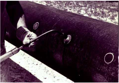
A2.0 Heat-Sink Capacity Method

A second method for predicting required head input levels was developed concurrently at EWI and involves measuring the ability of the flowing contents to remove heat from the pipe wall using a simple field test (Figure A1). This test involves quickly heating a 20-in. (50-mm) – diameter area on the pipeline with an oxy-fuel torch to between 300 and 325°C. The time required for the area to cool from 250 to 100°C is then measured using a digital contact thermometer and a stopwatch. Six heat-sink capacity measurement trials are made and the average calculated. The average value is referred to as the heat-sink capacity of the pipeline. The heat-sink capacity value is used to predict the weld cooling rates using empirical relationships that were developed from data generated in the field and in the laboratory for a wide range of conditions.

With both of these methods, the predicted weld cooling rate is reported as a function of heat input for a given set of pipeline operating conditions (Figure A2). Limits on the weld cooling rates are established based on the maximum tolerable HAZ hardness predicted using previously-established empirical correlations and the anticipated carbon equivalent of the pipe material. Both of these methods allow welding parameters (i.e., heat input levels) to be selected based on anticipated weld cooling rates.

A3.0 Shortcomings of Existing Methods

The Battelle model, while having served the industry well, has a number of shortcomings. First, the finite-element meshes that are used by the model have a fixed number of elements, so when the thickness of the materials of interest increases, the mesh becomes unacceptably coarse. This effect begins to occur at thickness of about 0.5 in. (12.7 mm) or so. Since burnthrough risk is negligible for pipe wall thickness of 0.25 in. (6.4 mm) and greater, this does not affect the burnthrough risk prediction capabilities of the model. In terms of weld cooling rates, however, an unacceptably coarse finite-element mesh produces results that are very conservative with regard to hydrogen cracking risk.

The second shortcoming of the Battelle model is the way in which hydrogen cracking risk is predicted from weld cooling rate predictions. For an individual run, the model uses the predicted weld cooling rate to identify a material carbon equivalent for which welds made under the conditions of interest will have a HAZ hardness less than a fixed value of 350 HV. This may be very conservative for some applications and non-conservative for others.

A4.0 PRCI Thermal Analysis Model for Hot-Tap Welding

The PRCI Thermal Analysis Model for Hot-Tap Welding is web-based and takes full advantage of existing on the Hub, a cloud platform. The model uses a proprietary finite-element solver that was developed at EWI. Mesh generation capabilities include sleeve, branch, and bead-on-pipe geometries (the latter for buttering layers and weld deposition repairs). Heat-sink capacity values can also be predicted for comparison with field-measured values.

A5.0 References

A1. Kiefner, J. F., Fischer, R. D., and Mishler, H. W., “Development of Guidelines for Repair and Hot-Tap Welding on Pressurized Pipelines,” Final Report – Phase 1, to Repair and Hot-Tap Welding Group, Battelle Columbus Division, Columbus, OH, September 1981.

A2. Shapiro, D. E., “Guidelines for Hot Tapping Pressurized Pipelines,” Research Report, Columbia Gas System Service Corporation Research Department, Columbus, OH, April 1984.

A3. Bubenik, T. A., Fischer, R. D., Whitacre, G. R., Jones, D. J., Kiefner, J. F., Cola, M. J., and Bruce, W. A., “Investigation and Prediction of Cooling Rates During Pipeline Maintenance Welding,” Final Report to American Petroleum Institute, December 1991.

A4. Kiefner, J. F. and Fischer, R. D., “Repair and Hot-Tap Welding on Pressurized Pipelines,” Symposium during 11th Annual Energy Sources Technology Conference and Exhibition, New Orleans, LA, American Society of Mechanical Engineers, PD-Vol. 14, pp. 1 – 10, January 1988.

A5. National Energy Board (Canada), “In the Matter of an Accident on 19 February 1985 near Camrose, Alberta, on the Pipeline System of Interprovincial Pipe Line Limited,” National Energy Board Report, June 1986.

A6. Kiefner, J. F., “Investigation of Cause of Failure of 14-Inch Pipeline at Mile Marker 21.09,” Final Report to Sun Refining and Marketing Company, Battelle Columbus Division, Columbs, OH, December 1986.

A7. Cola, M.J., Kiefner, J. F., Fischer, R. D., Jones, D. J., and Bruce, W. A., “Development of Simplified Weld Cooling Rate Models for In-Service Gas Pipelines,” Project Report No. J7134 to A.G.A. Pipeline Research Committee, Edison Welding Institute, Kiefner and Associates and Battelle Columbus Division, Columbus, OH, July 1992.

A8. Graville, B. A. and Read, J. A., “Optimization of Fillet Weld Sizes,” Welding Research Supplement, Welding Journal, April 1974.

A9. Kiefner, J. F. and Fischer, R. D., “Models Aid Pipeline Repair Welding Procedure,” Oil & Gas Journal, March 7, 1988.

A10. Bruce, W. A., Li, V., Citterberg, R., Wang, Y.-Y., and Chen, Y., “Improved Cooling Rate Model for Welding on In-Service Pipelines, ” PRCI Contract No. PR-185-9633, EWI Project No. 42508CAP, Edison Welding Institute, Columbus, OH.

Appendix B: Heat-Sink Capacity Measurement Procedure

Equipment Required:

• Chalk or soap stone
• Oxy-acetylene torch with “rosebud” tip
• Digital contact thermometer
• Stopwatch

Procedure:

1. Determine the direction of fluid flow.
2. Using chalk or soap stone, scribe three 2-in.-diameter circles (approximately 12-in. apart) on both sides of the pipe.
3. Starting with the downstream circle, use the gas torch to quickly heat the entire region to 300°C (572°F) using a circular motion. The maximum temperature should not exceed 325°C (617°F).
4. After attaining a temperature of between 300 and 325°C (572 and 617°F), remove the torch and apply the contact thermometer to the center of the circle.
5. While holding the thermometer in contact with the pipe, using a stopwatch, measure and record the time required to cool from 250 to 100°C (482 to 212°F).
6. Repeat Steps 3, 4, and 5 on the next untested upstream circle on the opposite side of the pipe. IF the pipe is still warm from the previous measurements, wait until normal temperatures are restored.

Once the measurements are complete, calculate an average time from the recorded readings.

Appendix C: Validation Data for PRCI Thermal Analysis Model for Hot-Tap Welding

C1.0 Introduction

The PRCI Thermal Analysis model for Hot-Tap Welding was validated by comparing model predictions to experimental data generated during a previous PRCI-sponsored program at EWI and to predictions made using the existing Battelle model. Examples from this validation exercise are given in the following sections.

C2.0 Validation Data

C2.1 Cooling Rate Prediction Capability

The cooling rate prediction capability of the PRCI model was validated using data generated during a previous PRCI-sponsored program at EWI. During this program, weld cooling rate data was collected over a wide range of wall thicknesses, natural gas flow rates, and welding heat inputs. This data was compared to predictions made using the PRCI model and the existing Battelle model. Examples of the results are shown in Figures 1 through 4. The results indicated that the Battelle model predictions tend to be non-conservative for thin-wall materials, particularly at low flow rates, and very conservative for thick-wall materials. The PRCI model predictions tend to be relatively accurate, with a consistent level of conservatism across wall thickness range.

C2.2 Burnthrough Prediction Capability

Since there is no comprehensive validation data for inside surface temperature, PRCI model predictions were compared to predictions made using the existing Battelle model for the conditions described above. Examples of the results are shown in Figures C5 through C8. The results indicate that, provided that the user enters a value for heat input only (i.e., allows the software to select specific values for welding current, voltage, and travel speed according to the preset algorithm), the PRCI model predictions are nearly the same as Battelle model predictions. For thin-wall materials, the PRCI model predicts slightly higher inside surface temperatures than the Battelle model. If the user enters specific values for welding current, voltage, and travel speed, the PRCI model is able to predict the effect of current level (electrode size) on burnthrough risk that was discovered during another previous PRCI-sponsored program at EWI. 

C3.0 References

C-1. Cola, M. J., Kiefner, J. F., Fischer, R. D, Jones, D. J., and Bruce, W. A., “Development of Simplified Weld Cooling Rate Models for In-Service Gas Pipelines,” Project Report No. J7134 to A.G.A. Pipeline Research Committee, Edison Welding Institute, Kiefner and Associates and Battelle Columbus Division, Columbus, OH, July 1992.

C-2. Bruce, W. A. and Threadgill, P. L., “Evaluation of the Effect of Procedure Qualification Variables for Welding onto In-Service Pipelines,” Final Report to A.G.A. Pipeline Research Committee for PR-185-9329, EWI Project No. J7141, Edison Welding Institute, Columbus, OH, July 1994.

FAQ